How To Draw The Marginal Revenue Curve

Update: A similar explanation to the derivation of the Marginal Cost curve can be read here.

For most JC students taking Economics as an “A” level subject, the explanation of key concepts using theoretical diagrams can be a bane. The chief reason for this is that these diagrams are often drawn through sheer memorising, instead of understanding what they are drawing.

Amongst the most complicated diagrams “A” level students will be expected to draw, are those from the Microeconomics firm-related chapters, “Production and Cost” and “Firm Structures”. A usual example of such diagrams is shown as below.

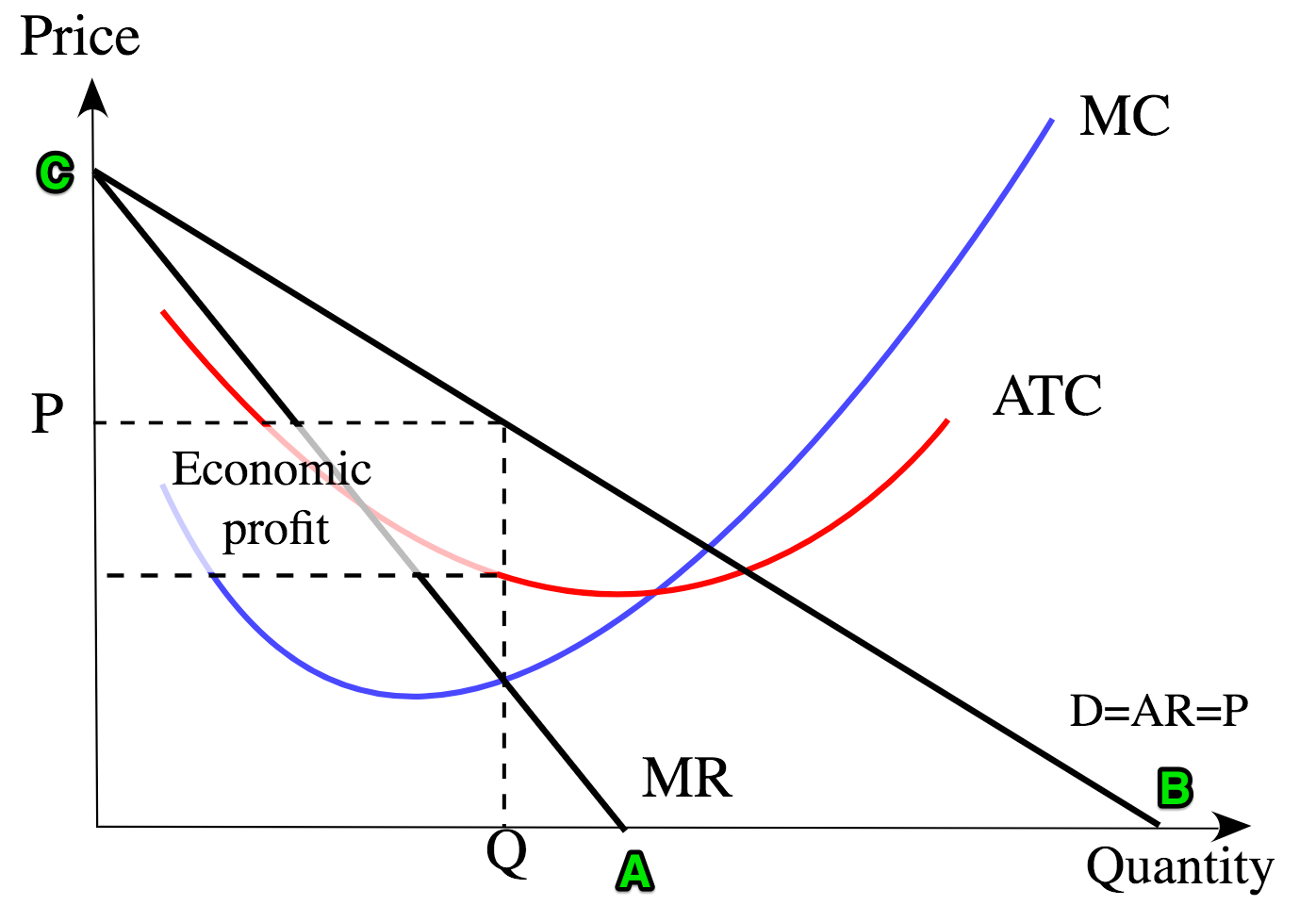
This is a typical diagram used to visualise the theory of “Production and Cost”. For today, we shall focus on the Average Revenue and the Marginal Revenue curves.

Average Revenue = The Total Revenue  of the firm divided by the total units of goods/services sold. Since the price for every unit sold is assumed to be the same, Average Revenue is then the same as Price for every given quantity demanded (i.e. both curves are the same here).

Marginal Revenue = The additional revenue gained from the firm selling the next unit of goods/services. Note what this implies is that the Marginal Revenue represents the rate of change of Total Revenue for the given quantity demanded.

The underlined statement is particularly important in understanding why the Marginal Revenue curve is drawn the way it is as above. Many students have drawn a wide variety of permutations when it comes to this diagram, and the key reason is lack of understanding.

Thankfully, students shouldn’t be too worried about having to draw their diagrams to microscopic accuracy levels because:

• Students are not expected to know the mathematical derivation of Marginal Revenue. However this is key to understanding the appearances of the curves as they are drawn, and I will explain how it’s done in the coming paragraphs.
• Drawing the MR in the proper fashion requires only knowledge of 2 easy points:
  1. The y-intercepts for both Average Revenue and Marginal Revenue are the same.
  2. The x-intercept of Marginal Revenue is exactly half that of Average Revenue.

Deriving Marginal Revenue Mathematically

If you recall, I mentioned that Marginal Revenue represents the rate of change of Total Revenue for the given quantity demanded.

Does this sound familiar to you? This in fact implies that Marginal Revenue is derived by the mathematical differentiation of Total Revenue with respect to Quantity.

Looking at the above diagram, the Average Revenue curve can be represented mathematically by the generic linear equation:

AR = mQ + C

Where m is the gradient of Average Revenue curve and C is the y-intercept of Average Revenue in the diagram. Q represents the Quantity Demanded.

Next, we derive the Total Revenue function:

TR = AR * Q = ( mQ + C ) * Q = mQ² + CQ

If we differentiate TR with respect to Q, we get:

MR = d(TR) / d(Q) = 2mQ + C

As with drawing lines in general, we only need 2 known points to derive the line.

The y-intercept of the Marginal Revenue curve is always the same as that of Average Revenue

Let’s put the AR and MR functions side-by-side:

AR = mQ + C   ;   MR = 2mQ + C

Did you notice that both share the same y-intercept, C?

So therefore on the diagram, the Average Revenue and Marginal Revenue curves always intersects on the y-axis.

The x-intercept of the Marginal Revenue curve is always half that of Average Revenue

Let’s put the AR and MR functions side-by-side again:

AR = mQ + C   ;   MR = 2mQ + C

Did you notice that the magnitude of the gradient of the Marginal Revenue curve is twice that of Average Revenue?

The result of this is shown on the diagram as B = 2A.

Do draw the Marginal Revenue curve with the above notes in mind

As above, 2 known points of the Marginal Revenue can be derived relative to the Average Revenue curve.

Students usually draw the Marginal Revenue curve as steeper than the Average Revenue curve, but they often neglect to draw the y-intercept and x-intercepts (i.e. both curves do not touch the axes), or when they do, the y-intercept and x-intercept are not drawn based on what we have discussed earlier.

To clarify, students will not be penalised for not drawing the diagram to such strict interpretations during “A” level exams.

That said, you would have to be asking for it if you make incredible mistakes, such as drawing the Marginal Revenue curve as above the Average Revenue curve during the exam!

In conclusion, knowledge of the derivation of Marginal Revenue is crucial in avoiding confusion when drawing this diagram, by consolidating strong foundations in studying for your exams.