Proof of Diminishing Returns in a Concaved PPC.

Curiously, some students struggle with getting the concepts behind the Production Possibility Curve (PPC) right.

And there are also others who claim to understand the various reasonings that went into the PPCs as drawn, but underestimate the challenge of constructing a PPC with high-quality details under exam conditions.

To be fair, I did take it for granted that constructing an arbitrary PPC wouldn’t be difficult. Especially if I drew free-hand, and used the excuse of drawing badly to fit somewhat not-to-scale data-points to the graph.

Here’s an actual example of a drawing that I did on the fly for a student just last week:

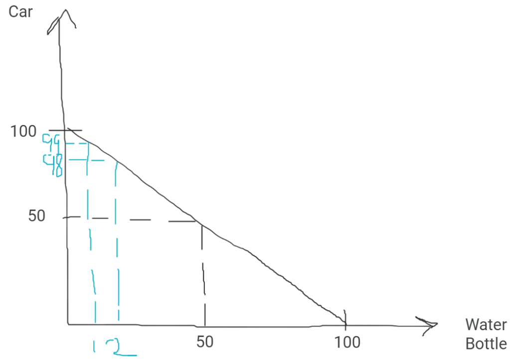
With the luxury of time, it becomes possible to see if it was possible to create a set of numbers that would allow ease of drawing the PPC – and that shall be the purpose of this article today.

I shall assume that the PPC is familiar to you – if otherwise, you can read more about it here.

Setting up the PPC.

Often, it is tempting to jump straight into the drawing, and neglect the laying of foundations to the PPC that we are about draw.

As good practice, we should always start by constructing the example in such fashion:

1. There are only 2 goods produced in the economy: Bottles and Cars;
2. The resources and production techniques are fixed;
3. All resources are utilised fully and efficiently; and
4. The resources are not equally capable in the production of either goods.

The first 3 points are straightforward in understanding that our PPC here, maps out the boundary to all possible production mixes to the economy.

It should also be mentioned that these conditions require that the PPC be drawn as a strictly-decreasing function. Otherwise it becomes possible to produce more of one good with an increase in production of the other, violating the must for trade-offs with full resource employments.

The last point is the most intriguing, because it forces the PPC to take a concaved shape:

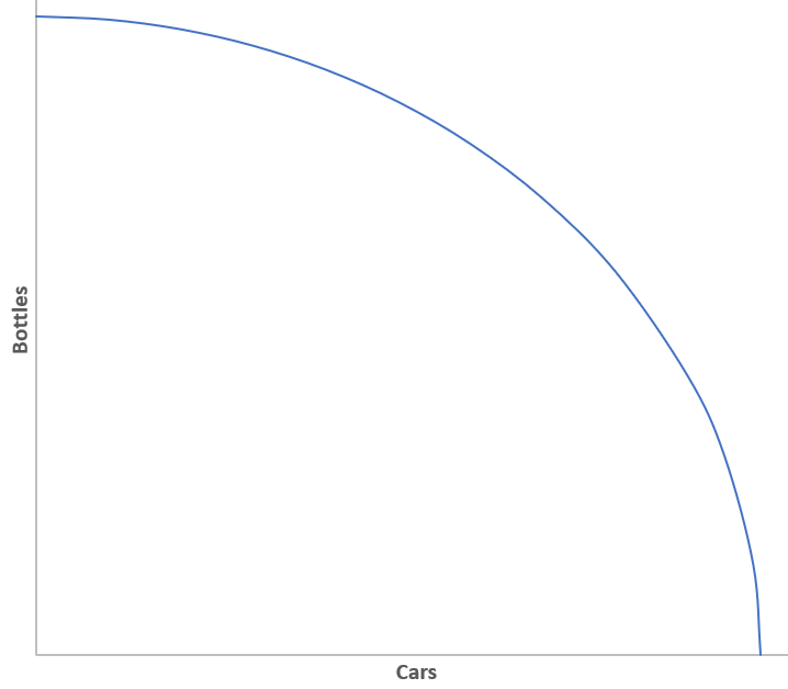
Why the typically-drawn PPC is concaved.

There are 2 main approaches to answering this question:

1. Bottom-up construction, and aggregation of output by individual resource for each possible resource allocation; or
2. Backwards deduction of each resources’ output capability based on the PPC as drawn.

Method 1 requires trial-and-error to illustrate the PPC well, since the curve is then constructed by discrete allocation choices by the economy.

On the other hand, Method 2 avoids this by allowing a good starting point from which each suitable resouce-combination can be mapped out. However, to do this very well, some mathematics is unavoidable as an arbitrary function needs to be constructed as a first step.

We will focus on Method 2 is the subsequent discussion as this is an opportunity to do that first step well, and make our lives easier in showing that the concaved PPC is the consequence of unequally efficient resources.

The mathematical representation of the PPC.

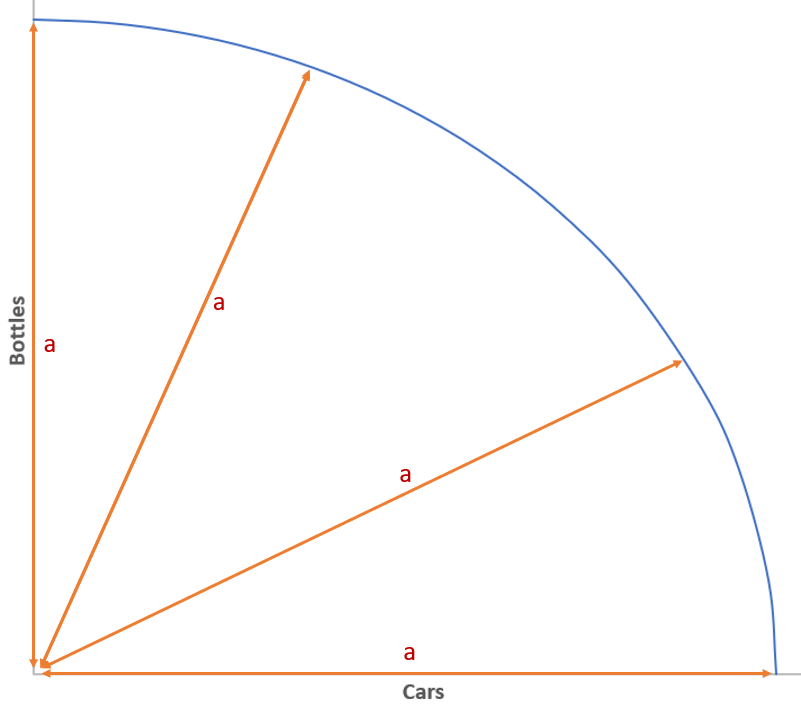
The easiest way to derive a function that would fulfill our needs, is to use a quadratic one, that also has symmetrical x and y-intercepts. In addition, we impose another requirement that: All points on the PPC being equidistant to the origin.

We can now utilise the Pythagorean Theorem to establish that the relationship between the x and y axes can be established as:

a² = x² + y²

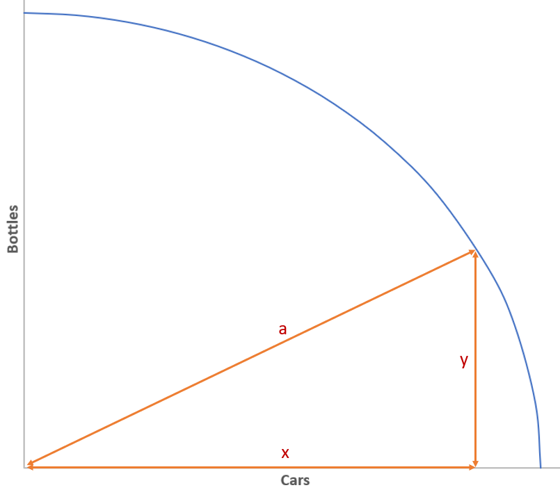
Making y the subject then yields us:

y = √( a² – x² )

Substitute “a” with 100.

To build our numerical example, we can map out a PPC using the above expression, by setting:

a = 100

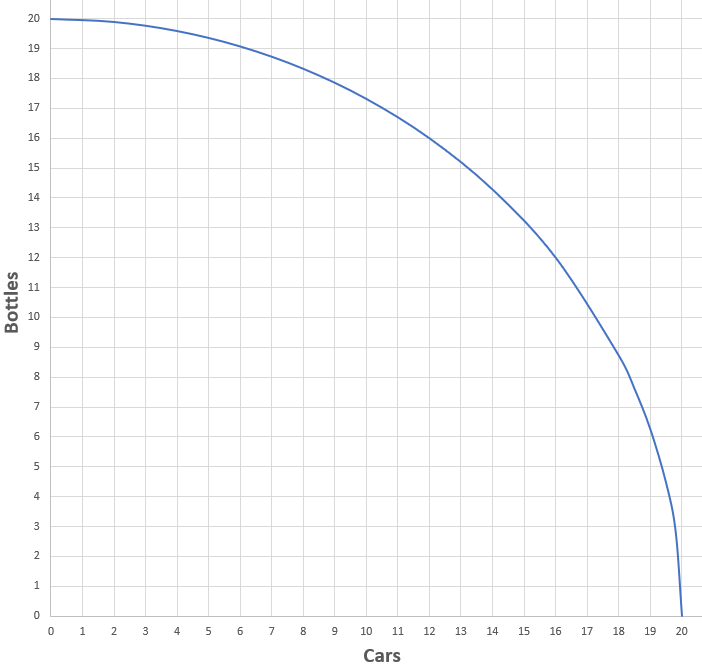
With our PPC as drawn above, it becomes possible for us to work backwards, and find specific production combinations that suitably represent each allocation of resource.

Specifically, we should look for points on the PPC that coincide with integer-combinations (i.e. at the intersection of grid-lines above):

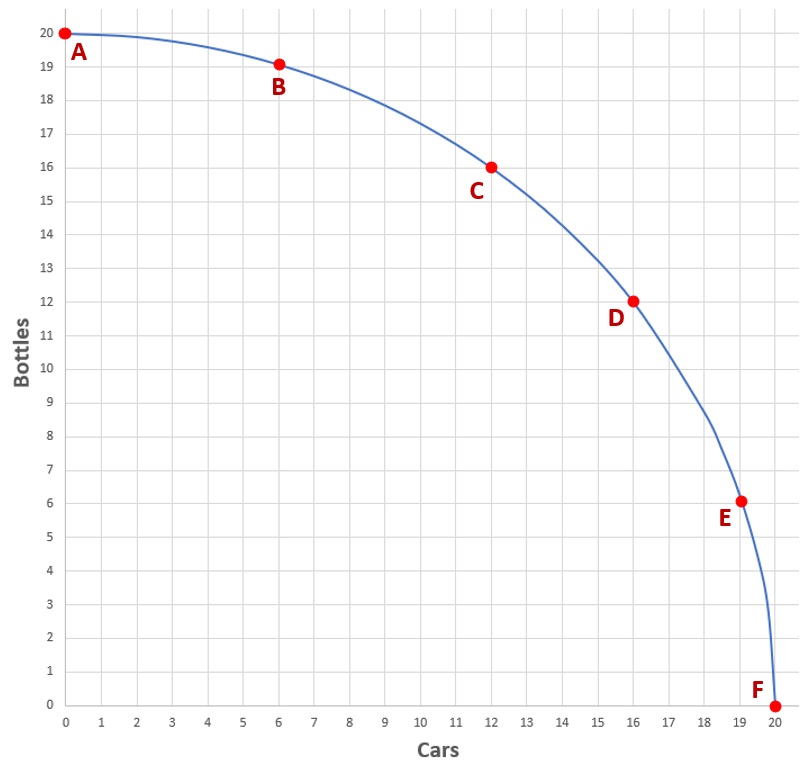
We can now work backwards based on the 6 points identified above, and conjure 5 people who are each capable of producing cars or bottles (but not simultaneously) to the following quantities:

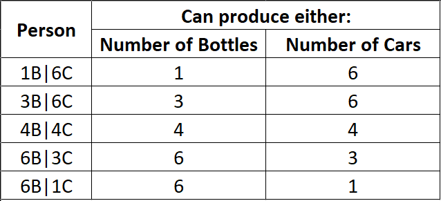
For subsequent ease of reference, each person is named after his/her production capacity in either good.

At a glance, we can see there is merit to constraining the PPC to symmetrical x and y-intercept, and having every point being equidistant to the origin: For each person, identified above, there exists a counterpart who produces the same quantities for each opposing good.

Now that’s a good start to making our lives easier for reproducing such examples for the exams.

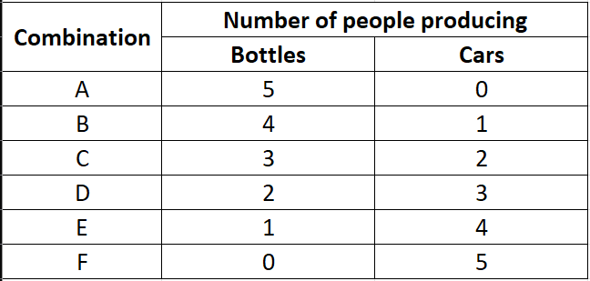
With 5 people that we can allocate to the production of each type of good, we yield 6 possible combinations:

Always maximising production.

The question now becomes: How should we allocate the people to each production point above?

Recall that the PPC maps out the maximum production levels at each combination – so therefore we should allocate the people on the basis of maximising the sum of bottles and cars produced at each point.

The easiest way to work out each allocation, is to start at either extremities (either producing bottles only, or cars only). For the purpose of subsequent discussion, we can start with bottles-only production:

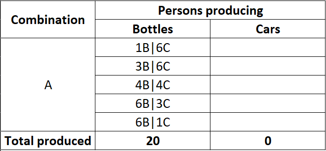
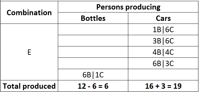
If we start producing cars, to fulfill our stated objective of maximising the sum of bottles and cars produced always, we should pick the person who is the least efficient in producing bottles and most efficient in producing cars.

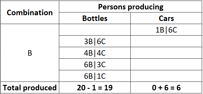
In other words, our choice of who we should re-allocate to the production of cars (from bottles), should seek to minimise the opportunity cost of producing each car for each next combination (i.e. the number of bottles lost for each car produced). Re-allocating Person 1B|6C to producing cars is the best option therefore:

We can apply the same logic for subsequent combination choices:

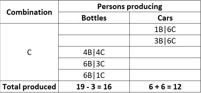
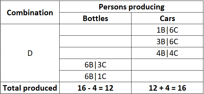
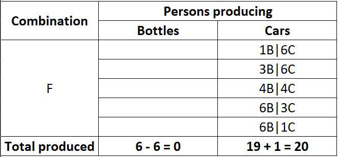
Notice that for each iteration, the opportunity cost of producing each next car increases? This implies diminishing returns, which is the result of:

1. Unequal efficiencies between producing either good for each resource; and
2. Always fully allocating resources for each production possibility such that the total production of both goods together is maximised.

Key takeaways.

A concaved PPC always exhibits increasing opportunity cost as production of a good increases at the expense of the other, for a given fixed level of resources that are fully employed.

In turn, increasing opportunity cost can be seen alternatively as diminishing returns.

We have therefore proven that a concaved PPC always reflects diminishing returns when producing more of a good, given a situation where resources are not equally efficient in producing either goods in the economy.

For students reading this, feel free to use the set of numbers utilised above for the exams. You can also reach out to me if you have questions, by leaving comments below, or PM-ing me here.