Explaining The Marshall-Lerner Condition In A Level Economics.

Most of us have seen applications of the Marshall-Lerner condition in Economics.

“By the Marshall-Lerner condition….” is how it usually goes.

But is it really important? In my years teaching Economics, students’ comments about the Marshall-Lerner have ranged from perfectly scripted explanations, to “huh, my teacher said it is not important”.

In fact, the Marshall-Lerner condition is very important in the Economics syllabus. And it will be my job to explain why and how it should be used.

And by the way, to put face to this rather important concept, here are the pictures of Alfred Marshall, and Abba Lerner, namesakes of the Marshall-Lerner condition:

The Marshall-Lerner (M-L) Condition

In Economics, we say that the M-L condition holds when the sum of the price elasticities of demand for exports and imports exceed 1:

PED_x + PED_m > 1

Determining whether the M-L condition is in force when analysing the effects of price changes to exports and/or imports is very important, as it will determine the outcome of these changes on the economy’s performance.

If you are interested in the mathematical derivation of this condition (which I promise you is not that complicated), you can take a look at the related wiki article.

When the M-L Condition Holds

What we are really interested in is the impact to the trade balance, and therefore the balance of payment, which is a key economic performance metric.

The trade balance (N) is represented by the difference between the export revenue of the country, and the import expenditure:

N = X – M, where X = P_xQ_x and M = P_mQ_m

Therefore:

N = P_xQ_x – P_mQ_m

If for example, an appreciation of the exchange rate occurs:

1. Export prices will increase and import prices will decrease.
2. The quantity demanded for exports will fall, and vice versa for imports.

Notice that when price increases/decreases, the corresponding quantity demanded decreases/increases, per the usual supply-demand analysis.

We can easily see this conundrum to the trade balance using vectors (in brackets):

N (?) = P_x (↑) Q_x (↓) –  P_m (↓) Q_m (↑)

And this is why the M-L condition is important – it gives direction to these sequence of events. 

Assuming that assumption holds now, we turn again to vectors, and represent higher-than-proportionate movements with double arrows:

N (↓) = P_x (↑) Q_x (↓↓) –  P_m (↓) Q_m (↑↑)

N (↓) = X (↓) – M (↑)

So therefore, given an appreciation in exchange rate, assuming the M-L condition holds, the trade balance (and therefore the balance of payments) will worsen.

The reverse is true for a depreciation in exchange rate – by reversing the vectors’ directions, we can conclude that the trade balance (and therefore the balance of payments) will improve.

When the M-L Condition Doesn’t Hold

Now this is the obvious anti-thesis to our analysis earlier. And you will see the importance of explicitly stating the assumption of the M-L condition whenever exchange rate movements are analysed.

If again, for example, an appreciation of the exchange rate occurs:

1. Export prices will increase and import prices will decrease.
2. The quantity demanded for exports will fall, and vice versa for imports.

Prior to applying the M-L condition:

N (?) = P_x (↑) Q_x (↓) –  P_m (↓) Q_m (↑)

But what if the M-L condition doesn’t hold in this case?

Then we get:

N (↑) = P_x (↑↑) Q_x (↓) –  P_m (↓↓) Q_m (↑)

N (↑) = X (↑) – M (↓)

So therefore, given an appreciation in exchange rate, assuming the M-L condition doesn’t hold, the trade balance (and therefore the balance of payments) actually improves, and vice versa for a depreciation in exchange rate.

Clearly the M-L condition plays a central role in determining the impact to the external economic performance of a country with exchange rate movements.

But what does the empirical evidence have to say on the M-L condition?

Enter the J-Curve Effect

One of the key determinants of the price elasticity of demand is the length of time elapsed.

Broadly speaking, this is because a shorter period of time elapsed gives less opportunities for the economic agents to react and adjust, compared with a longer period of time.

Therefore, in the short-term, the M-L condition is unlikely to be met as the demand for exports and imports will be more price inelastic.

Whereas in the long-term, the M-L condition is more likely to be met as the demand for exports and imports becomes more price elastic.

This situation is commonly depicted in the “J-Curve Effect” diagram:

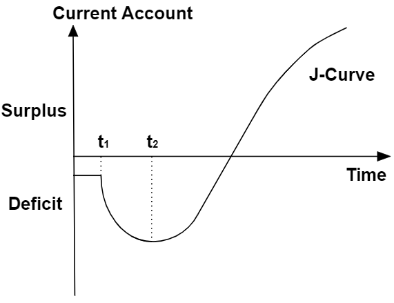
In this example, the country is experiencing a current account deficit at Time = 0.

Following textbook Economics, a devaluation of currency is then applied at Time = t₁.

In the short-term, the quantity demanded for exports and imports respond less than proportionately to the changes in respective prices caused by the devaluation. Reasons for that include:

1. Consumers’ tastes and preferences need time for adjustments.
2. Suppliers’ may not be able to increase output easily at short notice (i.e. price inelastic supply).
3. Existing contracts may legally bind the transacting parties to the agreed future purchases.
4. In addition, contracts often stipulate then prevailing exchange rates as fixed payment terms, rendering the transaction parties insensitive to fluctuations in the exchange rate.

As a result, the M-L condition doesn’t hold initially, causing the current account to worsen, rather than improve as intended.

Eventually, after Time = t₂, as the economic agents adjust appropriately to the devalued exchange rate, the M-L condition comes to force and the current account begins improving with time, eventually stabilising at a new equilibrium.

The M-L Condition and the J-Curve Effect are Indispensable

So we know by now that the M-L condition, and the related J-Curve effect are important concepts in understanding the effects of exchange rate changes to the economy.

But in fact, I would go as far as to say that they are indispensable for students in the exams. 

Beyond the utilisation of the M-L condition as a key assumption behind the analysis, the J-Curve effect adds significant evaluation points when utilised as an “anti-thesis” (albeit short-term one) to exchange rate policies to give a more balanced essay.

So why not give it a try next time?

Lend your support!

I hope that you have enjoyed reading this article of mine. I am giving my time to sharing my knowledge and every bit of support means a lot to me! Do drop me a comment or share this article on social media with your friends.

To find out more about my services as a JC Economics tutor, visit my website here.