Questions on Cost Curves and Economies of Scale

Question:

I don’t understand my notes.

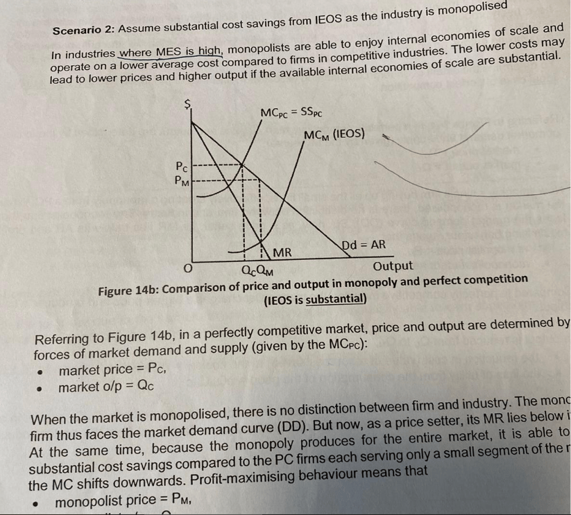
Referring to the graph and explanation below:

1. Why is the equilibrium price and output for the perfectly competitive firm where MC = AR? I thought the profit-maximising point for any producer would be where MC = MR?
2. I thought internal EOS will cause the equilibrium price/output to move along the AC curve. With the lowering of the MC as compared between the perfectly competitive firm versus the monopoly, wouldn’t that imply the AC curve shifted rather?

Ok, before I answer these questions directly, I would have to point out that I am going to assume you already know the concepts of cost conditions in Economics.

If you do not already, you can read more here.

My response to Question 1

A perfectly competitive firm is a price-taker as it is presumed to have negligible market power.

Also, due to perfect information and zero barriers to entry, each firm is presumed to face the same cost condition (i.e. same cost curves) in the market. This implies that MC_pc drawn in the diagram is representative for each of the perfectly competitive firms in the market.

Although perfectly competitive firms are presumably profit-maximising too, due to them being price-takers, the market “chooses” the equilibrium price/output for them – where supply meets demand (AR = MC_pc).

And now for Question 2

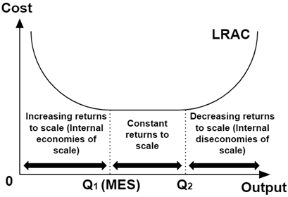
Internal EOS is defined as a situation where the AC falls (along the LRAC curve) as output increases for a firm.

Here we have a comparison between 2 different firms: A perfectly competitive one, and a monopolist.

There is no reason to assume that they would share the same cost condition – there is therefore nothing wrong with portraying each with differing MC curves.

It should be obvious that having 2 different MC curves, will imply that the associated AC curves will be different too.

How does that tie in with what students were taught – that internal EOS is illustrated with a movement along the LRAC?

The answer lies with the likely portrayal of short-run conditions in the diagram.

The LRAC is constructed by a series of SRACs, each corresponding to a level of fixed input (e.g. 1 factory, 2 factories etc):

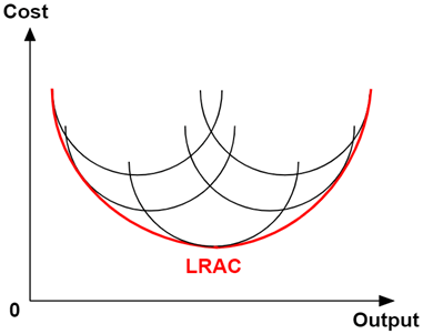
Marginal costs are based on changes to the total costs with each increase in output, which in turn vary depending on whether all factors of production are variable (i.e. short-run or long-run).

Under long-run conditions, we may presume that the AC curves would not differ between the perfectly competitive firm and the monopolist.

This is because they are in the same market and given similar cost conditions, it stands to reason that their respective cost of production differs only by movements along the same LRAC.

However, this particular diagram is likely portraying for short-run conditions.

How do we know?

Because each SRAC for similar firms, corresponds to each particular fixed input level. Therefore, due to the perfectly competitive firm being smaller, it will have an SRAC associated with a lower level of fixed input, and hence have an MC that will be higher than that of the monopolist at every output level.

Therefore internal EOS in this case then is portrayed by having a lower MC curve.

Do all these explanations matter then in my exam answers?

Not really.

Diagrams in Economics are ultimately tools utilised by students (and obviously educators), to bring across a particular point. How then you draw one should be customised accordingly.

Graphs are not “dead” objects!

In this case, the diagram on the notes shows that the price for a market when it is perfectly competitive is lower than if it was a monopolistic one, which implies cost savings for consumers (yay).

Although we had concluded earlier that the implicit assumption behind the graph is that it portrays for short-run conditions, the assumption is ultimately as what it says: implicit.

This differs from explicit assumptions, which are typically required for the detailed construction of more complex analytical frameworks (e.g. the long list of assumptions required for the Theory of Comparative Advantage).

Still confused? A good rule-of-thumb would be to follow the explanations in your school’s notes (it should boggle you if this doesn’t work).

As always, if you have questions, feel free to ask me, or leave comments below!