How To Draw The Kinked Demand Curve.

Although not a key part of the “A” level Economics syllabus, more than a few students have asked for an explanation behind the graph depicting “sticky prices” (more on that shortly).

The Premise.

In the Oligopolistic market structure, students are taught that producers tend to be loathe in competing on the basis of price – if they can help it. For the uninitiated, you can read more about this here.

In some cases though, it might well be inevitable, particularly in the case of extremely homogenous goods and services, since there is little or no scope in product differentiation. But that would be another story for another time.

The classic theory behind “sticky prices”, which describes the reluctance of producers in adjusting prices, asserts that producers in the Oligopolistic market will avoid:

1. Increasing price – Since there is risk that others will not do the same, which will cause hemorrhaging of sales volume; or
2. Decreasing price – Since there is risk that others will do the same, which will cause little, if any improvement to sales volume.

To put another way, when producers:

1. Increase price – They will face a price elastic demand curve, which will result in loss of revenue instead; or
2. Decrease price – They will face a price inelastic demand curve, which will result in loss of revenue too.

The Kinked Demand Curve.

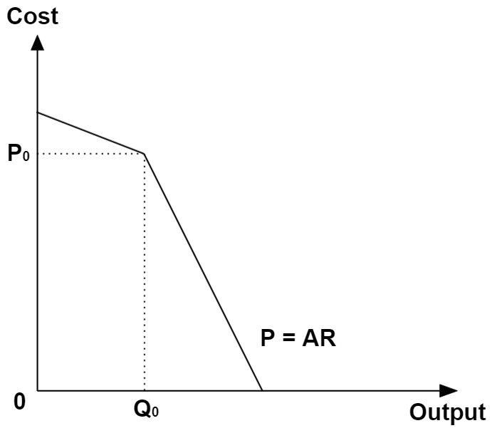
Having a demand curve whose magnitude of price elasticity of demand exceeds “1” when prices are higher than current price, and is less than “1” can be illustrated as such with the Average Revenue (AR) curve:

Deriving the MR Curve.

Because we need to find the profit-maximising point of Marginal Cost (MC) = Marginal Revenue (MR), we are obliged to illustrate the MR curve on the same diagram, deriving it from the AR curve.

This is probably the most confusing part of the illustration for many students, as the AR curve is discontinuous.

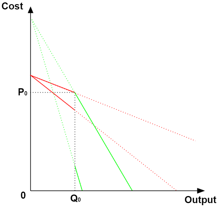
Importantly, you should be aware that the discontinuity occurs at Q₀, rather than P₀. This is due to the fact that both AR and MR are described at “each level of quantity”, rather than at “each level of price”.

The key implication to this, is that the respective MR derived for either sections of the AR are “sliced” vertically, rather than horizontally, as illustrated with their respective colours (red and green). Recall also that the MR curve always falls twice as fast as AR:

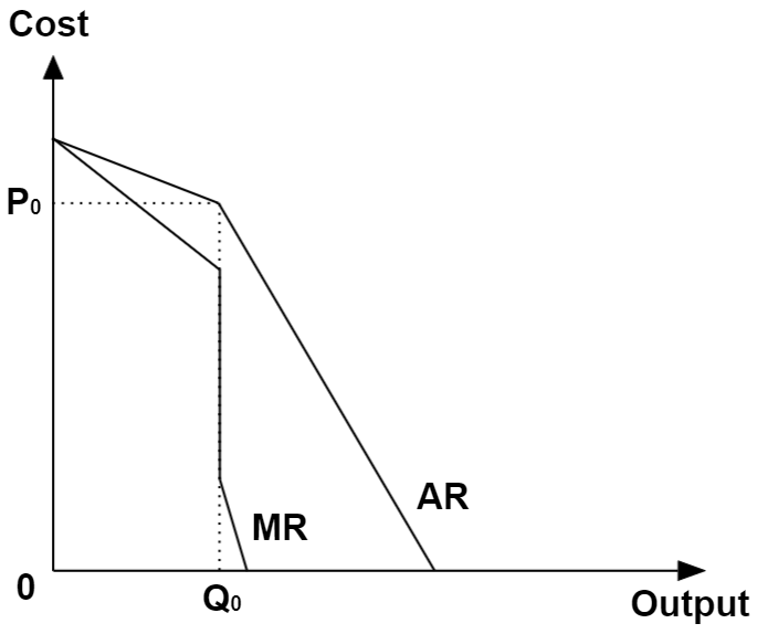
Removing the dotted lines that show the irrelevant portions of both sets of MR and AR will yield the final AR and MR:

Showing price stickiness.

Finally, we can show the firm’s profit-maximising output and price to be P₀ and Q₀, by conveniently adding MC to the diagram on the vertical portion of the MR curve:

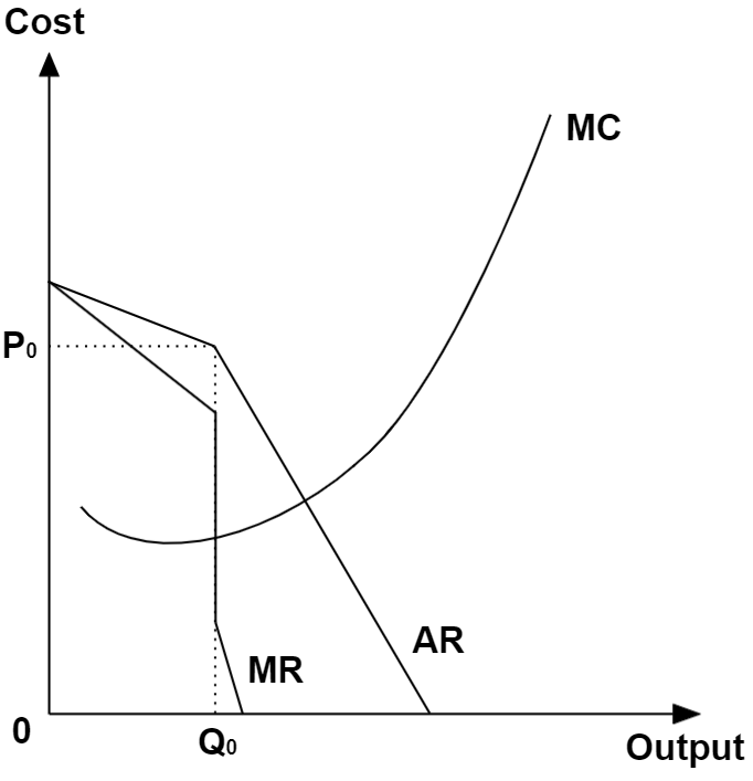
It should be fairly obvious now, with the above illustration, that as long as MC cuts MR anywhere on its vertical section, the equilibrium price and output will always be P₀ and Q₀.

This proves price stickiness given differing price elasticities as described earlier.

In particular, we can see that as long as MC is between MC₊ and MC_– below, cutting MR anywhere on the green band, the equilibrium price and output doesn’t change:

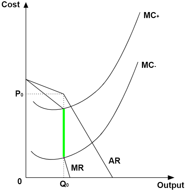
Accordingly, it would take very significant cost changes for the firm to adjust its price and output. Otherwise for most part, the firm would absorb changes to its operating cost without adjusting its price and output.

Interestingly, it can be observed that the green band (i.e. the tolerance for changes to MC), expands with the difference in elasticities between both sets of demand. This is an intuitive prediction as the more extreme the respective price elasticities get, the greater the revenue loss associated with adjusting price.

Try proving this on your own by following the steps above and drawing for more extreme price elasticities in demand!

Relevance of the Kinked Demand Curve

Simply speaking, it isn’t that much relevant.

In practical terms, the relative complexity of illustrating the Kinked Demand Curve coupled with the fact that a descriptive explanation as elaborated in the first part of this article works as well, makes it hard for students to justify spending time and effort illustrating this framework in the exams. Especially if you are pressed for time (which is always the case anyway).

In addition, the elephant in the room is the fact that the Kinked Demand Curve takes the current price and quantity to be a given, as a starting point for the construction of the model. This greatly weakens its explanatory efficacy as a model attempting to explain observed peculiarities in firms’ price and output decision.

Finally, as if it isn’t clear enough, the “A” level H2 Economics syllabus explicitly indicated that the reproduction of the Kinked Demand Curve in the exam is unnecessary, back in 2017.

Although not mentioned again in subsequent years’ syllabus, it can be construed that “saying it once is enough”.

Most schools, if they even mention it at all, have elected to tuck the explanations to the Kinked Demand Curve model in the “supplementary” section of their notes.

For most students, it may as well be marked as “irrelevant for exam” altogether, and so I will leave it as that with a detailed explanation as above, for the curious souls out there.