Why Is The AD-AS LRAS Vertical?

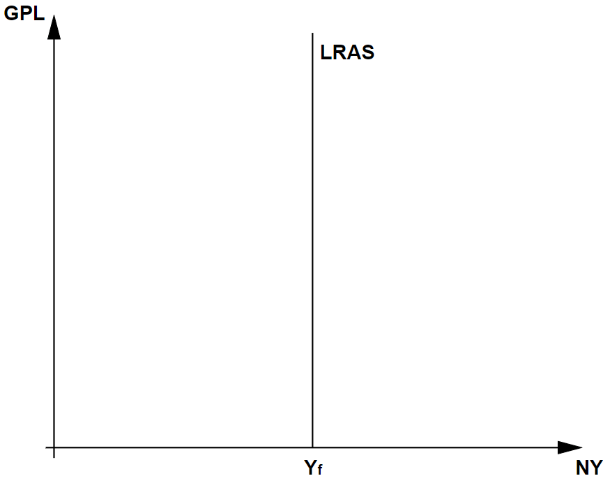
In the basic classical model for the Macroeconomics aggregate demand (AD) and aggregate supply (AS), the Long-Run Aggregate Supply (LRAS) curve is depicted to be vertical:

One of the most common questions I get from IB Economics students is about why the LRAS in the classical AD-AS model is vertical. Although many textbooks offer explanations on it, they tend to be short, highly varied, and generally less informative than they should be.

However, understanding why the classical AD-AS depicts a strictly vertical LRAS is important in enabling us to understand how this characteristic carries major implications on macroeconomic policy guidance.

What is the vertical LRAS?

The aggregate supply (AS) in Macroeconomics, simply refers to the aggregated supply of all goods and services produced by the economy. The AS curves in the AD-AS model illustrate the relationship between the produced output, against the economy’s general price level (GPL).

The LRAS is quite literally, the long-run counterpart of the Short-Run Aggregate Supply (SRAS). The differentiation in time period is determined by the defining assumptions that:

1. The short-run period is one where factor prices are inflexible; and
2. The long-run period’s factor prices are perfectly flexible.

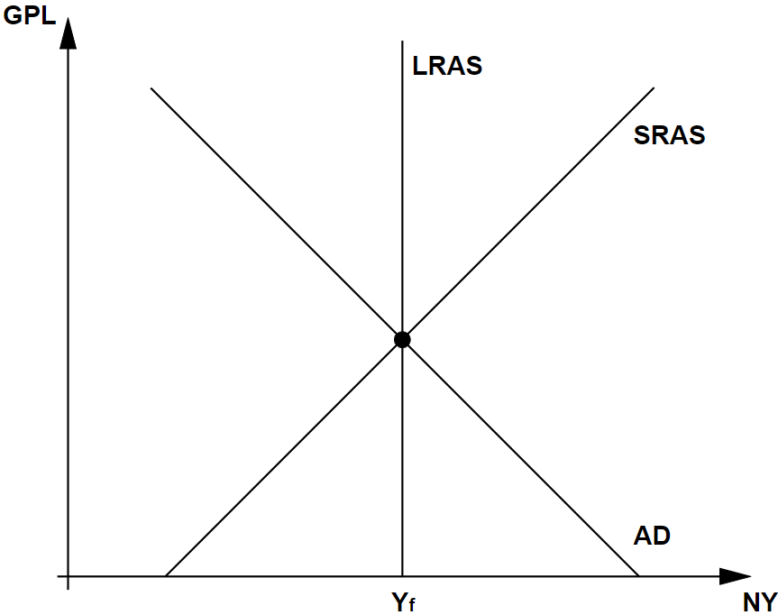
In the classical AD-AS model, the SRAS and LRAS curves are depicted as upward-sloping, and perfectly vertical respectively, suggesting that:

1. In the short-run, producers respond to higher GPL by increasing output; and
2. In the long-run, producers stick to a particular output level irrespective of any movements to the GPL.

It follows that because the short-run period dictates the given economic state at any point in time, whereas the long-run period governs the expected economic state in long-term equilibrium, then:

1. The SRAS defines the actual output level; and
2. In the long-run equilibrium, the SRAS’ solution in determining output is constrained by the need to adhere to the LRAS’ set of output solutions (i.e. the output must be where SRAS cuts LRAS).

Because of the market-clearing condition, the equilibrium output must be where the aggregate demand (AD) equals the aggregate supply (AS). Consequently, the long-run output level in the classical AD-AS model must occur where the AD, SRAS and LRAS simultaneously intersect:

Why is the LRAS vertical?

A vertical LRAS describes an aggregate supply that is perfectly price inelastic over the long run, i.e. producers are completely unresponsive in output decisions to changes to general price levels (GPL).

So this question can then be interpreted as “why are producers unresponsive in output decisions to price changes over the long run with fully adjustable factor prices“?

The short answer is that factor prices, at each given output level, will always adjust in the same direction and magnitude as the GPL over the long-run. Let’s consider a case where:

The GPL increases.

In the short-run, the given factor prices for each level of output remain unchanged, so a higher GPL would induce producers to increase output to maximse profits.

To fully understand why, we will need to revisit a key concept about profit-maximisation from Microeconomics:

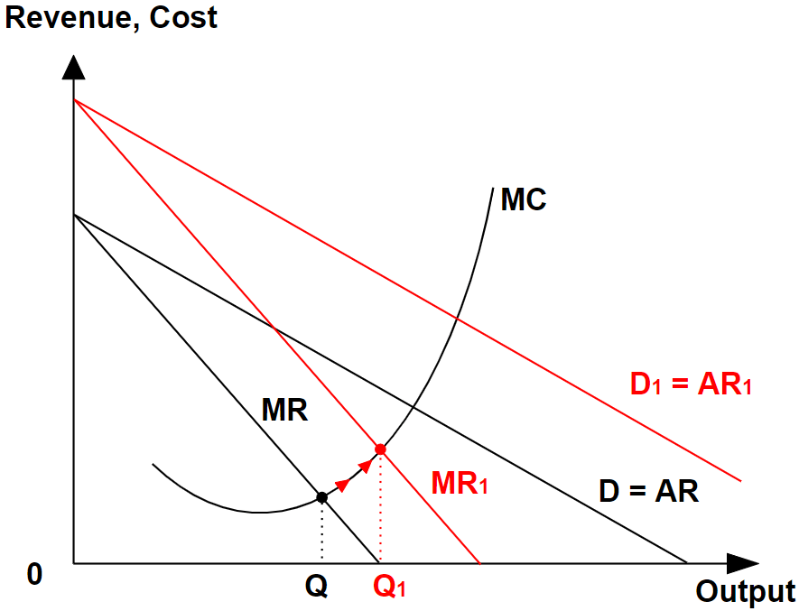
An individual firm maximises its profits where its marginal cost meets its marginal revenue (MC = MR in the diagram above).

For a firm observing higher prices to its good or service with no change to its cost structure, its MR will increase to MR₁. Because MR > MC at the original quantity of Q, the firm can increase its profits by increasing its output to Q₁, where MC = MR₁.

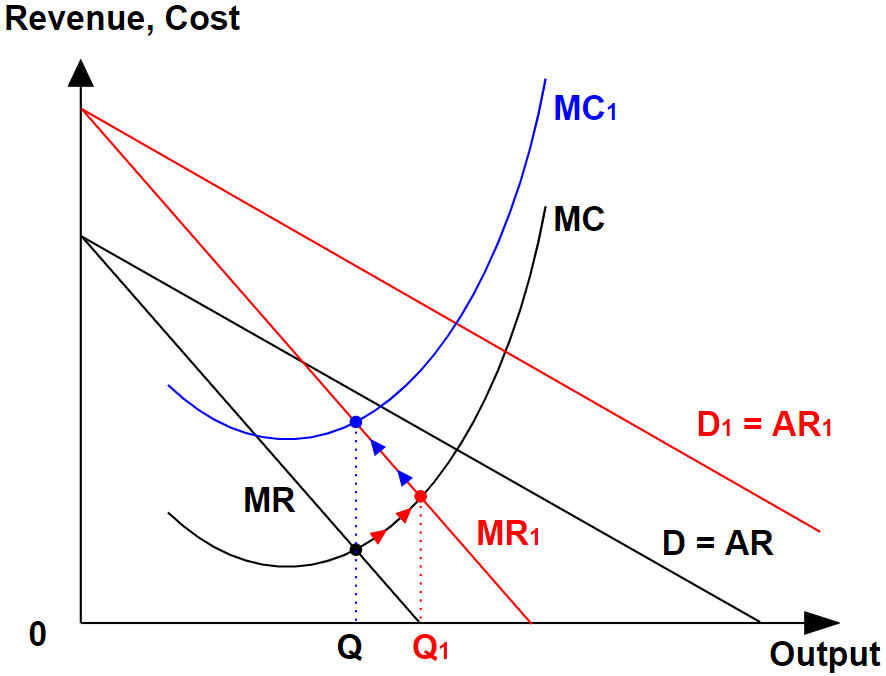
However, in the long-run, when factor prices can adjust, the MC will eventually increase to MC₁. This is because as the individual firm demands more factor inputs to increase output, factor prices will increase in the factors’ market, causing factor prices increasing at every level of the firm’s output.

The end-result is Q₁ falling again back to the original Q (MC₁ = MR₁):

Extending the above logic to the macroeconomic level, the assumption of perfectly flexible factor prices in the long-run therefore causes output to remain at Y_f despite higher GPL:

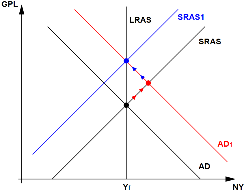
The above should look familiar to IB Economics students, because the vertical LRAS is in fact a consequence of the automatic adjustment process that results from any change to the AD. In this case:

1. AD increases to AD₁; and then
2. SRAS decreases to SRAS₁.

The extension of microeconomics logic to macroeconomics reflects the fact that the AD and AS are in fact aggregated demands and supplies of all firms in the economy.

You can apply the above analysis for the reverse case of GPL falling, to confirm that the output is always the same in the long-run irrespective of any changes to GPL indeed.

The significance of the LRAS output.

The LRAS, as constructed above, suggests that SRAS will always adjust in response to changes to AD in such way that output will always be the same in the long-run.

This constant output level (Y_f in the diagram) is commonly described as the full-employment output level because when factor prices are perfectly flexible, the owners of the factor inputs are assumed to seek maximum returns by maximising the employment of their resources:

1. Unemployed resources can be utilised by lowering factor prices to increase their attractiveness to firms; and
2. Overutilised resources can seek better returns by increasing factor prices, and return to a sustainable long-run employment level.

The significance of the LRAS’ full-employment output level therefore reinforces the classical AD-AS model’s vertical LRAS since that output level reflects the productive capacity of the economy, and its tendency towards it over the long-run.

How does LRAS respond to changes to SRAS?

Another common source of confusion for IB Economics students, lies in exam questions requesting for an impact analysis on changes originating from the SRAS.

A quick reminder: Supply curves reflect costs of production because they indicate the willingness and ability of firms to supply – which is based on costs of production after all.

Taking the example of a case where factor inputs have become cheaper over the long-run, SRAS will increase to SRAS₁ due to lower costs of production. Because a permanently lower cost of production for a given level of resource endowment in the economy results in higher productive capacity, LRAS will also shift to LRAS₁:

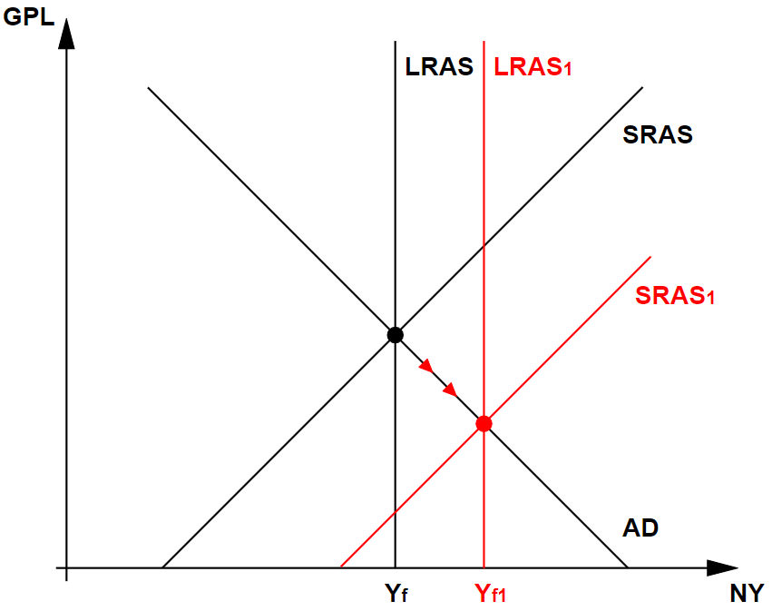
Therefore a persistent shift to the SRAS, results in a shift to LRAS to reflect changes to the economy’s productive capacity, and therefore shift the full-employment output level from Y_f to Y_f1.

LRAS still remains vertical though, because the changes to SRAS do not change the fact that the economy will always tend to produce at its full-employment level of output in the long-run for a given production state.

In other words, after SRAS changes and stabilises at the new level, and LRAS follows, GPL changes can only be triggered by changes to AD. As we had established earlier, changes to AD will not change output in the long-run (i.e. the new LRAS will also be vertical).

And it’s a wrap!

Leave your comments below if you have inputs or questions to my explanation as above.