Why Do Firms Produce Where Marginal Benefit Equals Marginal Cost?

Every year without fail, I will have students asking me: “I thought the output of the firm occurs at the point where demand meets supply?”

The confusion begins when students are told that the Marginal Cost curve can be considered to be the supply curve (since the cost of producing the next unit of good determines the price at which the supplier is willing and able to sell at).

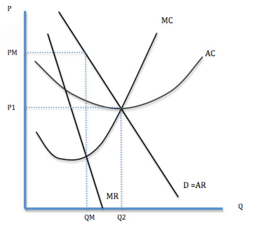
And then basing their understanding on foundational chapters such as “The Theory of Demand and Supply”, students then conclude that the point of output is where the “Supply” meets “Demand” (point Q2, P1 in the graph above).

Unfortunately in the Theory of Market Structure, this is incorrect, and many students have paid the price for this misunderstanding.

As always, understanding concepts trump confused rote learning. So let’s try to understand what is going on from here!

Differentiating between the Market Graph and the Firm Decision Graph

The first step to clearing up the confusion about the actual output level of firms, involves understanding that this graph actually explains the firm-level output and price level:

This firm-level diagram is used to illustrate the theory behind how the firm(s) decide on their price and output levels.

The graph below on the other hand, depicts the market-level output and price:

This market-level diagram is used to illustrate the price and output level across the market, and more importantly, doesn’t seek to explain firm-level decisions in price and output level.

Crucially, students should understand if the question is asking about the general market, the market-level graph should be utilized. 

Conversely, if the question relates to firm-level decisions, the firm-level diagram should be utilized. (E.g. when discussing about the virtues of the different market structures).

Why do firms produce at the point where MR = MC, and not where P = MC?

We have earlier established the fact that when it comes to pricing and output decision for firms, the firm-level diagram is more appropriate than the market-level one.

When discussing about the firm-level decision, students must know that firms produce at the point where MR = MC, which is not necessarily where P = MC.

To understand why, we must first define MR and MC:

• MR (Marginal Revenue) refers to the additional revenue gained from selling an additional unit of good/service.
• MC (Marginal Cost) refers to the additional cost incurred in producing an additional unit of good/service.

Now let’s explore the following 2 scenarios:

1. If MR > MC (i.e. LHS of the intersection point), the producer should produce the next unit of good/service because there is profit to be gained (additional revenue > additional cost).
2. If MR < MC (i.e. RHS of the intersection point), the producer should not produce the next unit of good/service because a loss will be incurred (additional revenue < additional cost).

Taken together this means that:

1. As the firm increases output in the initial phase, it produces on the left side of the point where MR = MC on the firm-level diagram
2. Therefore MR > MC and the firm has the incentive to produce more.
3. The firm stops increasing its production when MR = MC, because beyond this, the firm will suffer loss on the additional unit produced.

Therefore the profit-maximising firm should produce at the point where MR = MC.

The corresponding price at which the firm will sell, is found by looking for the corresponding price at which the buyer is willing and able to purchase (Pm in the above firm-level diagram).

When firms are not perfect price-takers, Allocative Efficiency is not achieved.

A key takeaway from the above exercise, is that with the exception of the Perfectly Competitive market (D=P=MR=AR), the market will tend to be Allocatively Inefficient. 

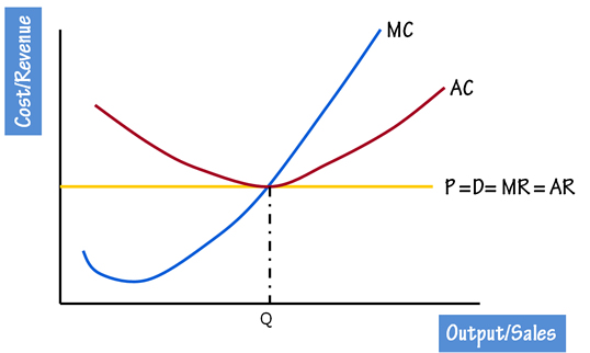
A quick review of the Perfectly Competitive market diagram shows that MR = P at all output levels. 

Thus the point where MR = MC, is also the point where P = MC.

A market is generally considered to be Allocatively Efficient when P = MC. Therefore the Perfectly Competitive market is Allocatively Efficient.

Since all other types of market structures have a diverging Marginal Revenue compared to Price, the actual output level can almost always be expected to be lower than the optimal output level for society, generating a dead-weight loss.

An intriguing question therefore arises:

Why do we generally refer to the Free Market as Allocatively Efficient when the Market Structure theories suggest otherwise?

This confusion occurs because we usually learn from earlier chapters that the Free Market leads to Allocative Efficiency by default, as the market will produce at the point where supply meets demand.

In fact, a key assumption that is seldom stated explicitly at “A” level Economics, is that the Free Market is presumed to be Perfectly Competitive, unless otherwise stated.

A good understanding of the use of these concepts is key to utilizing these theoretical frameworks well, adding value to our answers in the exams.

Students should therefore take note of this implicit assumption when studying to avoid confusion.

I hope that you have enjoyed reading this article of mine. I am giving my time to sharing my knowledge and every bit of support means a lot to me! Do drop me a comment or share this article on social media with your friends.

For more information about my services as a JC Economics tutor, do visit my website here.