All About the Law of Diminishing Marginal Returns

Some time ago, we had discussed on the derivation of Marginal Revenue in an earlier article, and showed its relationship with Total Revenue. Today, we will be building on the earlier discussion, this time focusing on the Law of Diminishing Marginal Returns and what they mean for the Firms’ cost and revenue. 

A major motivation for this article came from recent lessons with my students on Firms’ cost and revenue decisions. I have observed that many students are weak in their understanding of what appears to be a particularly abstract theory on firm behaviour. 

Granted, it didn’t surprise me much. As a student many years ago, I had generally disliked and avoided this particular topic during exams as well. It is admittedly difficult to visualise this topic for the uninitiated and unless explained well and clearly, this aversion would usually remain for a long time. 

As a highly experienced tutor now, it is possible for me to look back now and see how I could have improved my understanding of the Firms’ cost and revenue decisions. I use these techniques to help my students, and I am about to share them with you today, and hope that you will find it as useful as I have. 

What is the Law of Diminishing Marginal Returns? 

According to the Law of Diminishing Marginal Returns, as a firm increases its production of goods and services by increasing its variable factor inputs, there will reach a point where the increase in output decreases. This level of output and beyond, is said to be subject to Diminishing Returns. 

If this sounded confusing, don’t worry! There is fortunately an easy way to identify the point of Diminishing Returns based on the above definition.

In fact, the point of Diminishing Returns occurs when the Marginal Product begins to decrease. It really is that simple.

Why does Diminishing Marginal Returns happen?

Diminshing Marginal Returns happen because the factors of production are ultimately not perfectly substitutable.

A rational firm owner attempting to increase his output by increasing his labour force for example, would hire the most suitable candidates at each hiring exercise. Unfortunately, there is limited talent pool, and eventually he will be forced to hire sub-optimal workers, which ultimately slows his production gains.

Intuitively as well, hiring too many units of variable inputs for the given fixed inputs ultimately results in inefficiencies in production. As they often say, too many cooks spoil the broth.

As you might have noticed earlier, I had made mention of “fixed inputs” in the earlier sentence. Fixed inputs only exist in the short-run period. Students should note that the Law of Diminishing Marginal Returns is strictly applicable only for the short-run. 

A very common mistake made by students is to apply the Law of Diminishing Marginal Returns to long-run periods as well. A similar effect on the Long Run Average Cost is in fact termed “Diseconomies of Scale”. Do take note!

Illustrating the Law of Diminishing Marginal Returns

This is where students often get stuck in explaining what the Law of Diminishing Marginal Returns is, in the exams.

The best way to explain the Law of Diminishing Marginal Returns is through the use of a numerical example and a graph with corresponding cost and revenue curves.

Have a look at the following table, which illustrates the effect of increasing the variable input (labour in this case), on the cost and revenue of the firm.

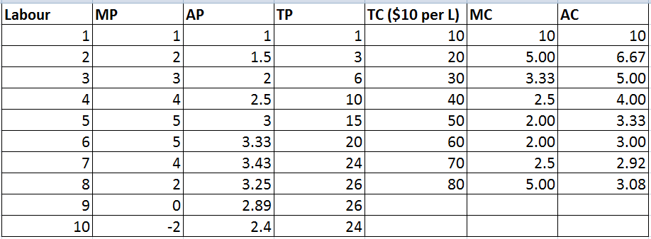
To create the above table, the following values were arbitrarily set:

1. Labour – Each row in the table represents the associated productions and cost for that quantity of Labour. 
2. Cost Per Unit Labour – Set arbitrarily at $10. 
3. Marginal Product (MP) – The additional output associated with the per unit increase in Labour. The Marginal Product is set intentionally to increase at the beginning, taper off, and then decrease, to illustrate the Law of Diminishing Marginal Returns. 

Lets look now at how we derived the other values from the above set of arbitrary values:

1. Total Product (TP) – Cumulative sum of the Marginal Product as Labour is increased. 
2. Average Product (AP) – Division of Total Product by the associated amount of Labour. 
3. Total Cost (TC) – Cost per unit Labour multiplied by the associated amount of Labour. 
4. Average Cost (AC) – Division of Total Cost by the associated Total Product. 
5. Marginal Cost (MC) – The gain in Total Cost as Labour is increased, divided by the associated Marginal Product. 

Observing the Law of Diminishing Marginal Returns. 

Referring back to our earlier discussion of the Law of Diminishing Marginal Returns, we had earlier determined that the point of Diminishing Returns occurs when the Marginal Product begins to decrease as Labour increases.

Looking at the above table then, the point of Diminishing Returns occurs at Labour = 6, where the Marginal Product is just about to decrease from 5 to 4. Correspondingly, the Marginal Product is also at its maximum point here. Also, the Marginal Cost is at its lowest point there as well.

To further illustrate the effects of the Law of Diminishing Marginal Returns on the firm’s production and cost, let’s now plot our data-points on a couple of graphs. Let’s start with the production curves:

Does this look familiar to you? This is how the Total Product, Average Product and Marginal Product curves are derived. They are not figments of imagination like how students often draw during exams, but actual data points!

Notice that the maximum point of the Marginal Product curve occurs approximately at Labour = 5 instead of at 6. This is because the data-points in our table are discretely divisible (i.e. widely spaced), as opposed to being infinitely divisible, and the curve (drawn using MS Excel) is actually a best-fit line for our data-points.

The representation of the table on the graph would improve if the increments to Labour was 0.1 instead of 1, but obviously this would make the creation of the table (especially in exams) cumbersome.

Observe also that as the Marginal Product dips, it eventually intersects with the Average Product at its maximum point. Students should pay special attention to this relationship between the Marginal Product curve and the Average Product curve, and reproduce this in the appropriate graphs in their exam.

The graph can be broken up into 3 main phases – Increasing Returns, Constant Returns and Diminishing Returns:

The Law of Dminishing Marginal Returns is now clearly illustrated by the graph, showing the 3 phases a firm can expect to experience as Labour is increased.

1. Until approximately Labour = 5, the firm experiences Increasing Returns, where the Total Product is increasing at an increasing rate, and Marginal Product is increasing. (Green area)
2. At approximately Labour = 5, the Total Product increases at a constant rate, and the Marginal Product no longer increases. This is the phase of Constant Returns. (Yellow area)
3. Beyond Labour = 5, the Total Product starts to increase at a decreasing rate, before eventually decreasing. The Marginal Product is always decreasing from here. This is the phase of Diminishing Returns. (Red area)

Turning now to the cost curves: Similarly, this graph can be broken up into: Increasing Returns, Constant Returns and Diminishing Returns, which we have done above.

Let’s also zoom in on the Average Cost and Marginal Cost curves for a better view.

Again, because the curves drawn are best-fit lines as earlier explained, you might have noticed that the minimum point of the Marginal Cost curve occurs approximately at Total Product (Quantity) = 20 instead of at 17.5. For the purpose of the following discussion, we will take reference from the graph instead as well.

The Law of Dminishing Marginal Returns is also now clearly illustrated in this set of graphs, showing the 3 phases a firm can expect to experience as output increases:

1. Until approximately Marginal Product = 20, the firm experiences Increasing Returns, where the Total Cost is increasing at a decreasing rate, and Marginal Cost is decreasing. (Green area)
2. At approximately Marginal Product = 20, the Total Cost increases at a constant rate, and the Marginal Cost no longer decreases. This is the phase of Constant Returns. (Yellow area)
3. Beyond Marginal Product = 20, the Total Cost starts to increase at an increasing rate. The Marginal Cost is always increasing from here. This is the phase of Diminishing Returns. (Red area)

Observe also that as the Marginal Cost increases, it eventually intersects with the Average Cost at its minimum point. Students should pay special attention to this relationship between the Marginal Cost curve and the Average Cost curve, and reproduce this in the appropriate graphs in their exam.

Explaining the Law of Diminishing Marginal Returns for the ‘A’ level exam. 

All of the above might seem intimidating, especially the creation of the table and then illustrating it on the graph. Don’t worry! Here is a suggestion on how you may explain the Law of Diminishing Marginal Returns during the exam.

1. Define broadly what the Law of Diminishing Marginal Returns means. (Marginal Product starts decreasing) 
2. Explain the basis and principles behind this theory. (Imperfect substitution of factors of production) 
3. Create the numerical example in table form (I used 10 rows in this example, but in the interest of time, you can cut back on the rows while still showing the 3 phases of production discussed earlier). 
4. Draw the production and cost curves. 

Don’t be worried about having to match the graphs to the table you had drawn. To save time in the exams, you can draw the curves arbitrarily (but of course retaining at least the general shape of the curves), and then label the points separating the 3 distinct phases in the Law of Diminishing Returns, as the appropriate figures from your table. This avoids the problem of attempting to draw the curves “to scale”.

Lend your support!

I hope that you have enjoyed reading this article of mine. I am giving my time to sharing my knowledge and every bit of support means a lot to me! Do drop me a comment or share this article on social media with your friends.

To find out more about my services as a JC Economics tutor, visit my website here.