How To Draw the Marginal Cost Curve.

Every “A” level Economics student knows how to draw the “Market Structure” curves. Still, every year without fail, I find myself having to explain to them how and why the curves appear as they should.

I had previously written an article about how the Marginal Revenue (MR) curve is derived – and judging by the number of hits I am getting, it would appear that it is well-received. A quick leap of logic led me to conclude that I should do a similar piece for the Marginal Cost (MC) curve.

First, the MC curve’s shape.

As my students often gleefully note, it is shaped like the “Nike logo”. And for good reason.

The cost function of a well-behaving firm (by Economists’ standards) is dictated by the Law of Diminishing Marginal Returns, which states that:

1. At low output level, the firm enjoys increasing returns as output increases; and
2. At high-enough output level, the firm experiences decreasing returns as output increases.

For more details on the Law of Diminishing Marginal Returns, I had previously written about it here – so I will not be talking more about it here.

It can be seen that at Stage 1 above, the MC must be falling as output increases faster than Total Cost (TC), and vice versa in Stage 2, as output increases slower than TC.

A more rigorous approach utilising some Math easily proves this point:

1. The TC curve is represented as a cubic function;
2. Since the MC is the additional cost associated with the production of an additional unit of output, it can be derived from the differentiation of TC; and
3. Differentiating a cubic function gives a quadratic function: a.k.a the MC curve’s “Nike logo”.

The graphical representation of the above makes it clearer:

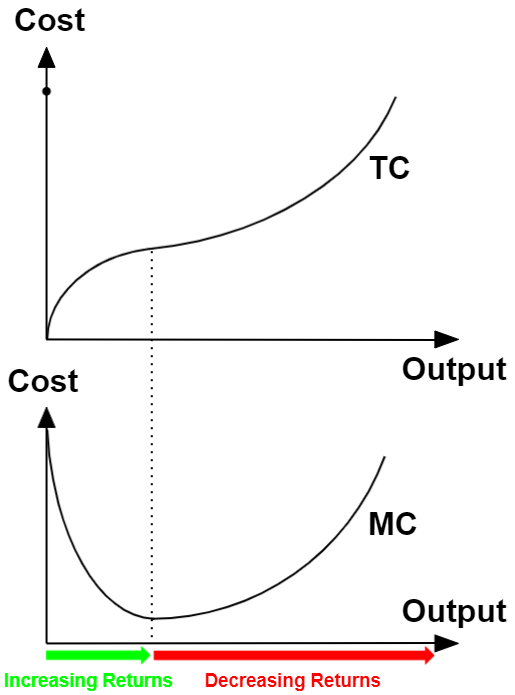
During the phase of increasing returns (green arrow), the TC curve flattens gradually as output rises faster than TC. Bring the result of differentiation from TC, and hence a representation of TC curve’s gradient, MC falls during this phase.

During the phase of decreasing returns (red arrow), the TC curve steepens instead as TC rises faster than output, causing MC to increase during this phase. It can be inferred therefore that the MC’s minimum point occurs when Diminishing Marginal Returns sets in.

MC cuts AC at its minimum point.

The second important aspect to the graphical representation of the MC curve, vis-à-vis the other cost curves in particular, is the fact that it must intersect the Average Cost (AC) curve at its minimum point.

The intuition behind it is not difficult thankfully. Consider how the MC interacts with AC by way of its incremental addition to TC:

1. If MC < AC: When the “new” AC is calculated incorporating the new additional cost into TC, it must be less than the previous AC calculated; and
2. If MC > AC: When the “new” AC is calculated incorporating the new additional cost into TC, it must be more than the previous AC calculated.

The mathematical representation of the above makes it clearer:

Difference between “New AC” and ” Previous = AC” = New AC – Previous AC

Where New AC = [ ( Previous AC * Q ) + MC ] / ( Q + 1 )

The condition of New AC > Previous AC can be represented by:

New AC – Previous AC > 0

Substituting New AC as a function of Previous AC yields:

[ ( Previous AC * Q ) + MC ] / ( Q + 1 ) – Previous AC > 0

Some simplification then yields the necessary condition:

MC > Previous AC

Try a similar proof yourself for the opposing condition of New AC < Old AC !

In summary, this is proof that when MC < AC, AC is falling (New AC < Previous AC).

And when MC > AC (i.e. has cut AC from the bottom), then AC is increasing (New AC > Previous AC).

MC cuts AC at its minimum point – the “atas” explanation.

Of course with my background in Economics/Math tertiary training, I couldn’t resist attempting a generalised continuous approach (as opposed to the discrete one above) to the proof.

To do this, first we represent the cost function as TC = f(Q)

Since AC = TC / Q , we can say that AC = f(Q) / Q

And since MC = dTC / dQ , then MC = df(Q) / dQ

We can find Q when MC intersects AC by solving for MC = AC :

df(Q) / dQ = f(Q) / Q

Unfortunately the expression cannot be simplified further satisfactorily, but thankfully, this suffices for our purpose, as we can alternatively prove by showing that the same expression repeats at the minimum point of AC.

We do this by differentiating AC:

d(AC) / dQ = ( df(Q) / dQ ) / Q – f(Q) / Q²

And then setting it to 0 to solve for Q at the minimum point of AC:

( df(Q) / dQ ) / Q – f(Q) / Q² = 0

Which then simplifies to:

df(Q) / dQ = f(Q) / Q

As we can see indeed, the expressions relating the intersection of MC and AC, and the minimum point of AC are the same, proving that both points coincide on the graph.

The End.