
The commonly accepted wisdom amongst Economics padawans is that when buyers are subject to information asymmetry biased towards sellers, they would offer an average price for the good or service.
Few texts go beyond explaining if “average” as used here quite literally means the mean value, or just vaguely meaning “somewhere in-between the extremes”.
Without having to resort to irrationality as white-washing to explain why there’s more than meets the eye, we can follow the thought process behind a certain Mr. Rational Average Joe, and uncover some nuances behind the buyers’ price determination when subject to imperfect information about the good or service.
Joe’s Purchase.
Joe would like to purchase a pair of earphones of a certain brand and model – the eponymous EP-1. Crucially, he decides that online shopping is the way to go, rather than visiting the manufacturer’s shop to learn more about the product (thereby eliminating strong signaling effects from the seller).
Now, anyone who has done their share of online purchases for electronics, will know that it is common for the products to be showcased as pictures by the sellers in uniformly boxed states. Like this:

Unfortunately (or fortunately) for Joe, because EP-1 has somehow gained the properties of open-source, there are many sellers of EP-1 with wildly varying prices not too different from the picture above, and showing their wares in similar pictures.
It doesn’t take much for Joe to realise that there is strong likelihood of him ending up with the purchase of a lemon EP-1 on the online marketplaces. A higher selling price is no guarantee against purchasing an EP-1 that is a sorry excuse of a manufacturer-grade one.
Or even one that has already seen the insides of others’ ears. Yuck.
Now, Joe may be Average.
But also trained in Statistics.
Joe has spent half a day looking up and down various online marketplaces, and concluded that few of the originally-manufactured EP-1 in mint condition (fetching the highest value of $100) are actually circulating in the market.
Indeed the degree of open-source was to such extent that Joe has determined that the value of all EP-1s sold follows a normal distribution, and the mean price was $50.
How realistic is that? I hear some asking.
Well in essence, a normal distribution is one where the observed values tends to cluster around a specific value, with equal likelihood of being greater or lower than that value. In fact, this describes the distribution for many real-world examples, which is why it is commonly used as a starting for many statistical analyses.
In any case, faced with only the same sanitised pictures of EP-1s from all the online sellers, Joe has little information on hand to inform him further.
He also has to assume that the market is very competitive, and therefore the prices offered by sellers represents the actual value of the EP-1s being sold on aggregate.
Alas, Joe can’t do better in the absence of more information, and can only hope that his conjecture that the competitive market space will cause sellers to balance between higher sales volume with lower prices, and higher profits per unit sold with higher prices is sufficiently correct.
Joe is also a pro at Microsoft Excel.
Joe’s sample of roughly a hundred offerings has allowed him to estimate the mean price ($50) and the standard deviation ($15) – key metrics required to construct a normal distribution function.
Using Microsoft Excel’s inbuilt normal distribution function, and iterating over 10,000 simulated EP-1 actual values, he constructs a normal distribution to the actual value of EP-1s sold.
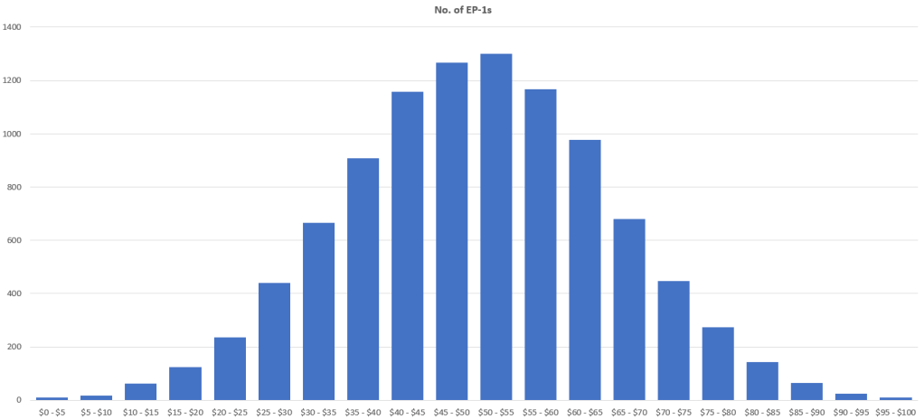
At a glance, we can see that the probability density is highest around the mean of $50. This may suggest that to maximise the probability of purchasing an EP-1 which has an actual value close to the purchase price, Joe should indicate a purchase price in that region.
This would agree with the common refrain mentioned at the beginning of this article, that when buyers are subject to information asymmetry biased towards sellers, they would offer an average price for the good or service.
But is this true?
There are 2 aspects to the solution of Joe’s purchase price problem:
- Joe is guaranteed to “over-pay” as sellers whose EP-1s are of higher true value will not entertain his purchase price; and
- The extent to the over-payment is uncertain until Joe has purchased and unboxed the EP-1.
At first glance, it might appear that Joe could purse pure risk minimisation as a strategy. But to see why that’s a rubbish solution, consider that the best solution would be to buy nothing, since a transaction guarantees some risk.
Another possible way to determine a solution would be to calculate the expected value of the EP-1 for a given purchase price, and choose one that minimises the expected over-payment. Unfortunately, it is well-documented that a naïve application of expected values to advise purchase outcomes has a tendency to be influenced unduly by outliers.
In particular, consider the following scenario separate from the main problem discussed so far: Joe gets a choice to participate in either of 2 lucky-draw games, both of which involving him sticking his hand in a box to fish out an EP-1 for his own:

Strictly applying the expected prize value on its own dictates that Joe would prefer Lucky Draw B over Lucky Draw A. Realistically though, Joe is probably indifferent between ending up with a lemon EP-1 worth $5 or $1. When it’s bad to the degree of non-usability as in both cases, Joe won’t care less about having to choose whichever lucky-draw game.
Intriguingly, this short example can provide inspiration for an acceptable strategy. Joe figures that he could, for each purchase price offered:
- Determine a threshold risk level that he can accept;
- Estimate the values of the EP-1s that meet his risk tolerance;
- Set a loss tolerance on the over-payment he is willing to accept;
- The optimal solution is then the highest purchase price that would fulfil the requirements of Point 1 and 3.
We can see how this works with an example, starting first with a “50-50” approach, where Joe is happy as long as the true value of the EP-1 purchased is within the top 50% of the EP-1s that sellers would be willing to sell to Joe, for his purchase price.
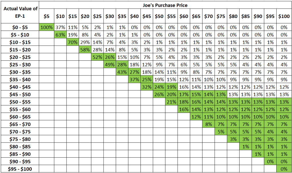
We start by mapping the probabilities in increments of $5 in purchase price, using the data-set Joe had created:

We can then indicate, in green, the sets of EP-1s that would make Joe happy for each given purchase price (i.e. within the top 50% in value):
Joe has decided that he is willing to accept having to pay up to $10 more than the true value. With that, we can see that the purchase price that enables at least a 50% probability that the EP-1 purchased would have a true value of no more than $10 off the purchase price occurs at $50:
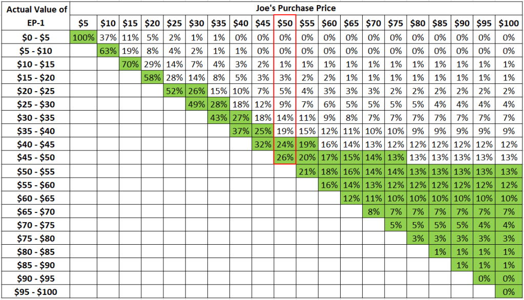
Incidentally, the solution to Joe’s purchase price selection is indeed similar to the “average price” assertion by many school texts to be selected by the buyer when faced with information asymmetry.
But clearly, we got there with clear specifications on its derivation. In fact, we can see as well, that the optimal purchase price for Joe is a function of his risk appetite.
Joe, the Risk-Averse.
Suppose Joe starts to get cold feet with a risk tolerance of 50%, and opts instead for a risk tolerance of 80% instead (i.e. he is more comfortable with a 80% probability of getting the EP-1 within the $10 loss tolerance):
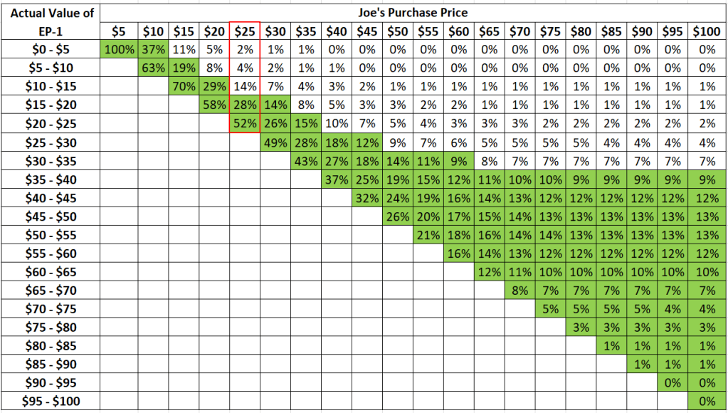
The optimal purchase price is then $25 – which makes intuitive sense because a lower purchase price should reduce risk exposure.
Joe, the Risk-Loving.
Suppose, Joe is instead, in the mood to indulge in the thrill of gambling, he can increase his risk tolerance by aiming for the top 10% in value for the EP-1s for sale at each purchase price.

As expected then, the optimal purchase price is now higher at $75.
It should be added also, that Joe’s risk appetite may also be reflected with the adjustment of the loss tolerance. Greater risk aversion can be effected with lower loss tolerance (e.g. reducing the tolerable variance in actual value of EP-1 purchased from the current $10, to $5).
Final Word
By now, it should be clear from Joe’s experience: The assertion that buyers, when subject to information bias against them, will pick the average price, is at best very simplistic.
What’s certainly true rather, is that the buyer will pick a purchase price that is within the estimated extremities of the good’s value. Exactly which price, depends strongly on the estimated distribution of the goods’ value, and the buyer’s risk tolerance.
Nor is this an abstract example in itself. Asymmetric information on the buyers’ part, has been implicated in many cases, as a major cause for market gyrations, such as in the case of cryptocurrencies.
Now that we have laid the foundation to how buyers respond to information asymmetry based on their risk profile, we can do a separate discussion for cryptocurrency, and see what factors make it particularly pre-disposed to sharp price movements, especially with new information or changes to market environment.


I never thought about it this way, thanks for providing a new angle.
LikeLike