
Judging by the number of hits I got for a similar article, “Why Do Subsidies Give Deadweight Loss?“, and repeated questions on how deadweight loss may be derived from various government interventions, it seemed timely for me to delve into such topic again, this time for price controls, starting with price floors.
What follows assumes that you are familiar with the broad concepts of a price floor. If you aren’t yet, read more about it from my free notes here.
A primer to Deadweight Loss
Deadweight loss refers to the loss of social welfare caused by market efficiencies – at least that’s how most books explain it.
But that’s a vague, and often unhelpful definition to live by, especially when attempting to quantify it on-the-fly in the exams. Here’s a more helpful way:
In a given market’s demand and supply, there must exist a market output level that exhibits the maximum social welfare level attainable. In the absence of market failure, this typically occurs where the market clears (i.e. where the supply meets demand).
To see why in more detail, you can look up the Marginalist Principle.
It stands to reason that an output level that deviates from that social-welfare-maximising output level, must result in a reduced social welfare level. Quantifying that reduction in social welfare level will give us the deadweight loss resulting from that output level.
In other words:
Deadweight Loss = Social Welfare max – Current Social Welfare
Where:
- Social Welfare max is a constant as determined by the given market demand and supply;
- Social Welfare = Producers’ Surplus + Consumers’ Surplus ; and
- Social Welfare max >= Social Welfare
If required, more details on the derivation of both consumers’ and producers’ surplus may be found here.
For purpose of subsequent analysis, Social Welfare max is illustrated as below, as the sum of the green (consumers’ surplus) and blue (producers’ surplus) areas:

The subsequent deadweight losses will then be calculated by subtracting the given social welfare, from the above areas representing maximum social welfare.
What the Price Floor looks like.
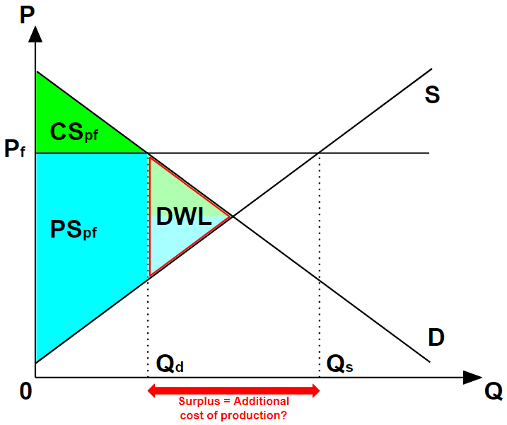
The typical price floor, in theory, results in an output surplus, because producers will be incentivised to produce more, while consumers will cut back due to the higher price, illustrated by Pf below:

In the absence of further interventions from the government, whilst producers produce up to Qs per the diagram above, they will not be able to sell past the quantity demanded, Qd. Consequently, producers’ revenue generation does not extend past Qd, so that even if they had produced at Qs, no additional producers’ surplus could be gotten beyond Qd.
Similar logic applies to the consumers too, so that the social welfare is reduced from the initial maximum level, resulting in a deadweight loss as illustrated in most textbooks:

At this point, astute students may realise that if producers are assumed to produce at Qs, which results in the output surplus pointed out above, there must exist additional costs of production that should count into the deadweight loss too:
Intriguingly, I have yet to come across any IB or “A” level Economics textbook or notes that make mention of this apparent discrepancy.
It can be assumed however, that as producers’ inventories pile up due to consumption < production, producers will eventually be forced to reduce production to Qd, which would conveniently explain away that additional cost of production that should have been added to the deadweight loss too.
Price floor with government purchase support.
Usually, a price floor is implemented to help producers gain more revenue through higher price (at the expense of consumers). For this to happen, the revenue gained from the higher price, must outweigh the revenue lost from a reduction in output sold (i.e. demand is price inelastic).
In many cases though, the government opts to purchase the surplus, especially if the good produced is durable and can be stored for extended periods of time. Superficially at least, this should guarantee a better outcome for producers as intended from the onset.
In our theoretical model, the government guarantees to purchase any amount of surplus produced, which allows producers to produce up to Qs. Doing so leads to the following additional outcomes:
- Producers gain producers’ surplus as they get to sell additional output of Qs-Qd; and
- The government’s expenditure spends Pf.(Qs-Qd) purchasing the surplus.
The implication of the first point is obvious enough: The producers’ surplus (solid blue area) increases up to Qs. But when it comes to the second point, since government expenditure cannot increase from thin air, it was to be funded by society and netted from its overall welfare.
Accordingly, we derive the new outcome to social welfare as below, by first:
- Increasing the total social welfare by increasing the producers’ surplus (solid blue area); and then
- Subtracting out the total government expenditure (outlined in red).

The final social welfare associated with a price floor accompanied by government purchase support, will then look like this:

Of the original social welfare pre-implementation of price floor, only the solid blue and green area (producers’ and consumers’ surplus respectively) remains. The rest were lost to the reduction of consumption level from the original equilibrium point, to Qd and counted towards deadweight loss (transparent blue and green areas bounded in red).
Area “b” was additional producers’ surplus gained by the expenditure of tax monies – so there was essentially no net gain or loss from the societal perspective.
In addition, the cost of the government expenditure that hadn’t been accounted for by the increase in producers’ welfare, needs to be factored into the overall social welfare, and is therefore represented as deadweight loss as well (solid orange area), in addition to the earlier deadweight loss explained.
Using mathematical representation as an alternative.
Whilst a step-by-step illustrative approach using the diagrams as above typically makes for clearer representation, arguably this may not always be the case for some of us.
Thankfully, we can use a more mathematical approach instead as an alternative, by first labelling the respective areas in the diagram, and then doing the necessary arithmetic:

******
Social Welfare max = Consumers’ Surplus max + Producers’ Surplus max
Social Welfare max = ( a + g + h ) + ( e + f )
******
Social Welfare pf = Consumers’ Surplus pf + Producers’ Surplus pf – Govt Expenditure
Social Welfare pf = ( a ) + ( b + e + f + g + h ) – ( b + c + d + e + h )
Social Welfare pf = a + f + g – c – d
******
Deadweight Loss = Social Welfare max – Social Welfare pf
Deadweight Loss = ( a + g + h + e + f ) – ( a + f + g – c – d )
Deadweight Loss = h + e + c + d
******
As can be seen, this is the same result as derived with the earlier approach. So students may indeed use either approach to arrive at the appropriate solution in deriving the deadweight loss for a given price floor.
Update (2026): The team at JC Econs 101 has also collaborated with DeadWeight·Plots to produce a step-by-step animation of the price floor diagram showing the deadweight loss and impacts to consumers and producers. Be sure to check it out!