Why Total Revenue Is Maximised When Demand Is Unitary Price Elastic.

A few practice “IB” Economics Paper 3 (quantitative assessment) and a few confused “A” level Economics students later, I concluded that I couldn’t take it for granted that my students can readily identify the maximum point of the producer’s total revenue on the demand-supply diagram, in Microeconomics.

In general, Total Revenue is maximised when:

1. The Marginal Revenue is $0; and
2. The demand is Unitary Price Elastic (i.e. Price Elasticity of Demand or PED = -1).

Fortunately, it is fairly easy to understand why intuitively, and mathematically.

Zero Marginal Revenue means no further increase to Total Revenue.

By definition, the Marginal Revenue refers to the additional revenue gained by the sale of one additional unit of good by the producer.

That also happens to describe the Marginal Revenue earned by producers as the first derivative of Total Revenue.

For reasons that I have described in great detail here, in general, the Marginal Revenue function shares the same y-intercept as the Average Revenue’s, but slopes exactly twice as fast downwards:

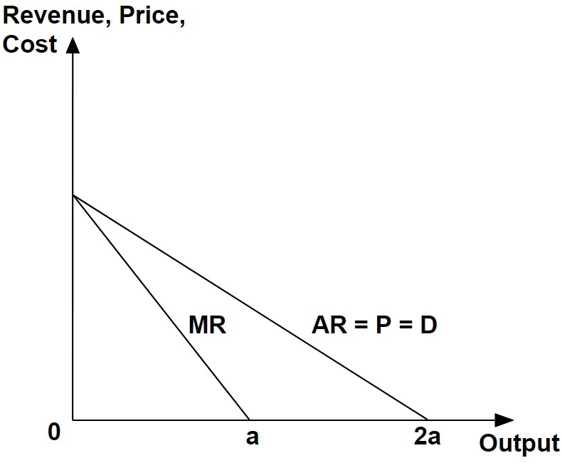
Because we generally assume that the producer sells each unit of good at exactly the same price, the Average Revenue must equate to Price at all levels of output. Also, mapping Price against Output necessarily describes the Demand function: Hence AR = P = D.

In terms of Total Revenue, since it is simply the product of Price and Output, 2 points can be readily identified from the above diagram:

1. When Output is zero (Output = 0 in the diagram), Total Revenue must be zero; and
2. When Price is zero (Output = 2a in the diagram), Total Revenue must also be zero.

In addition, recalling that the Marginal Revenue measures the increase in Total Revenue per additional unit of output:

1. The Total Revenue must rise as long as the Marginal Revenue > $0; and
2. The Total Revenue must fall as long as the Marginal Revenue < $0.

Therefore, the Total Revenue must max out at Marginal Revenue = $0 since the Marginal Revenue is a strictly decreasing function which eventually becomes negative, marking the point where Total Revenue must start to fall after it was increasing initially.

Those who are more mathematically-inclined will also recognise that a first derivative function that is linear (Marginal Revenue), and with a negative slope, implies that the original function (Total Revenue) must be a parabola with a maximum point at its single line of symmetry.

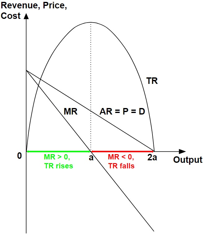
And thus the maximum point of Total Revenue occurs when Marginal Revenue is zero.

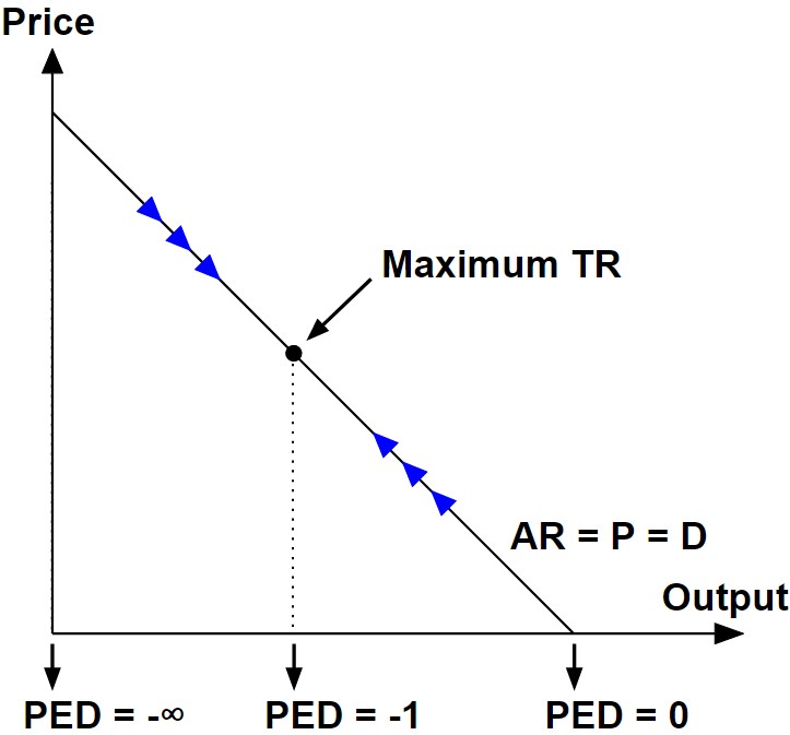
Revenue is maximised when demand is neither price elastic nor inelastic.

A common misconception amongst students is that the Price Elasticity of Demand (or PED) is static at all points of a given demand function, which isn’t true.

Consider the mathematical formula for calculating PED, which measures the ratio of the rate of change of quantity against that of price:

PED = ( ΔQ/Q * 100 ) / ( ΔP/P * 100 )

The above function can also be simplified and expressed as:

PED = ( ΔQ/ΔP ) * ( P/Q )

In the above expression, ΔQ/ΔP is the inverse of the demand function’s slope, and a constant (that is also negative) since the archetypical demand functions we encounter at “IB” and “A” level Economics are linear.

On the other hand, P/Q clearly decreases as output increases, beginning at ∞ when output is zero, and ending at 0 when price is zero. This also implies that the demand transits from being price elastic initially, to being price inelastic at some point – i.e. the demand is unitary price elastic at that point.

Recall that producers can utilise the prevailing value of the PED to determine the appropriate price (and output) level for increasing Total Revenue:

1. Reduce price (increase output), if |PED| > 1; and
2. Increase price (reduce output), if 0 < |PED| < 1.

For further clarity, you may read more about how price elasticity concepts work, from my free notes here.

It turns out that the strive for increasing Total Revenue from either sets of price and output movements as above, converges on the point of unitary price elasticity for demand, which implies also that maximum Total Revenue is achieved there:

Putting everything we have discussed up to this point together yields us a single point on the demand-supply diagram where the following are simultaneously true:

1. Total Revenue is maximised;
2. Marginal Revenue is zero; and
3. The demand is Unitary Price Elastic.

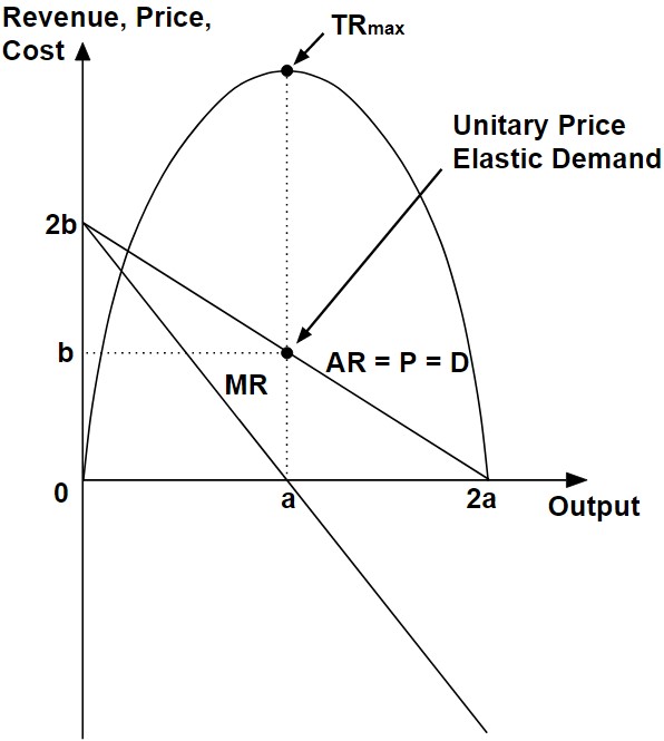
As a final demonstration that the above is true, we can show that the demand is indeed Unitary Price Elastic when the Marginal Revenue is zero, by utilising the following facts:

1. The Marginal Revenue is zero where the output is exactly half that of the maximum output that the producer is willing and able to produce (at zero price); and
2. The expression: PED = ( ΔQ/ΔP ) * ( P/Q )

We can then calculate the PED where the Marginal Revenue is zero based on the respective axes-intercepts of a and b:

PED_MR=0 = ( – 2a / 2b ) * ( b / a )

This can then be simplified to confirm a unitary price elasticity of demand:

PED_MR=0 = -1

Which proves conclusively that Total Revenue is indeed maximised where:

1. Marginal Revenue is zero; and which
2. The demand is Unitary Price Elastic.