
The standard Economics theory for IB and A-level Economics says that firms maximise profit where their marginal cost (MC) equals their marginal revenue (MR). This is a statement that the vast majority of students will take for granted.
And it’s not hard to see why, especially when both the MC and MR functions are presented in familiar graphical form:
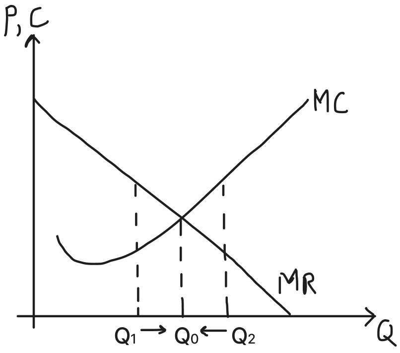
In this typical depiction, the MC function is a “Nike” curve that intersects the linear MR line exactly once. As an aside, more information about how the respective functions are derived and why they have these shapes can be found in my earlier articles about the fascinating math behind the MC function and the MR function.

The intuition behind why the profit-maximisation point occurs where MC=MR at Q0 is attractively easy to grasp too. As a reminder, the MR and the MC are defined as the additional revenue and cost experienced by the firm when it produces the next unit of the good respectively. Therefore, the profit-maximising firm currently producing at Q1 should increase output as there is net profit to be gained since MR > MC, and vice versa for the case of producing at Q2 since the opposite is true. The profit-maximising firm therefore produces at Q0 where MC = MR.
The Mathematical Proof
The firm’s profit-maximisation problem can be written as:
Where TR and TC are Total Revenue and Total Cost, respectively, and Q is the quantity of output.
We can start by writing the general equations for Average Revenue (AR) and Average Cost (AC):
Where α, b, c, d and e are constant coefficients.
Multiplying both by Q gives us:
Subtracting TC from TR gives the firm’s total profit, denoted by π:
Differentiating π with respect to Q gives the rate at which total profit changes as output increases:
Then set the derivative to zero to find the maximum value of π:
Now let’s derive MC and MR separately. Differentiating TC with respect to Q gives MC:
Differentiating TR with respect to Q gives MR:
As mentioned earlier, the profit-maximising firm produces at the value of Q which satisfies MC = MR:
Moving all the terms to the right-hand side and simplifying the equation gives:
This is, in fact, the same result obtained by setting the derivative of π with respect to Q to zero to find the maximum value of π.
A maximum or a minimum?
At first glance, the algebra seems to confirm the familiar rule that the firm maximises profit where MC = MR. But the first derivative of π with respect to Q is a quadratic function of Q. Setting it equal to zero can therefore give two distinct outputs where MC = MR.
In fact, this is supported by a more mathematically complete example of MC and MR depicted on the same graph:
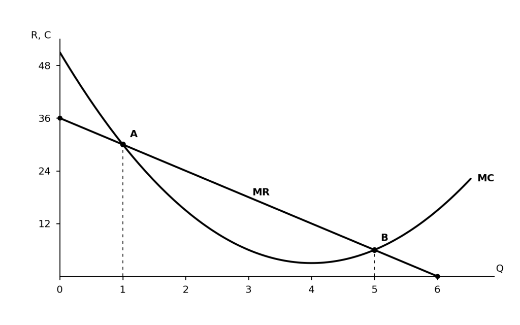
In this example, the coefficients are α = 1, b = −12, c = 51, d = −3 and e = 36. Substituting these values into the marginal cost and marginal revenue equations gives MC = 3Q² − 24Q + 51 and MR = 36 − 6Q.
Substituting the same coefficients into the total cost and total revenue equations, we get TC = Q³ − 12Q² + 51Q and TR = −3Q² + 36Q:
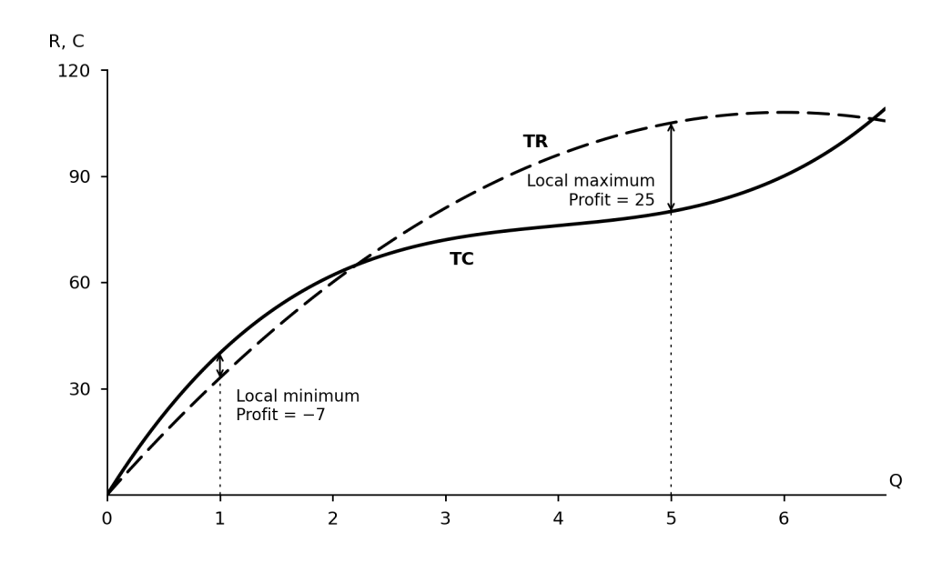
Thus we can visually identify that the minimum profit occurs at Q=1 where TC-TR (loss) is at its greatest, while the maximum profit occurs at Q=5 where TR-TC (positive profit) is at its greatest.
Plotting profits, π = TR – TC, against Q shows the local minimum and maximum even more clearly:
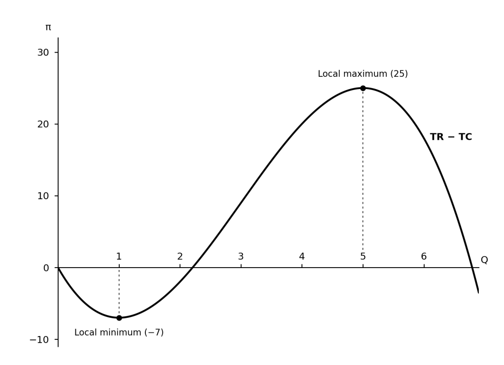
Why the local minimum?
Here’s the intuition: For as long as MC > MR, when Q is low, increasing Q ensures that the profit continues to fall, since doing so continues to add negative profit for every additional unit of the good produced.
When MC = MR and thereafter MR > MC, additional output increases profit since every additional unit of the good produced starts to add positive profit instead. Therefore, when MC crosses MR from the top, the producer earns the minimum profit.
It is therefore important for students to state clearly that the producer is profit-maximising when it produces at Q where MC crosses MR from the bottom, since MC < MR and profit is increasing as Q increases up until that point (local maximum).
Case of only maximum profit.
Astute students would recognise by looking at the MC and MR graph that there is nothing to stop us from raising TR aggressively, such that MC crosses MR only once, from below.
For example, decreasing d from −3 to −4 and increasing e from 36 to 63 gives MR = 63 − 8Q. The new MR curve starts above MC and crosses it from above only once, at Q = 6:
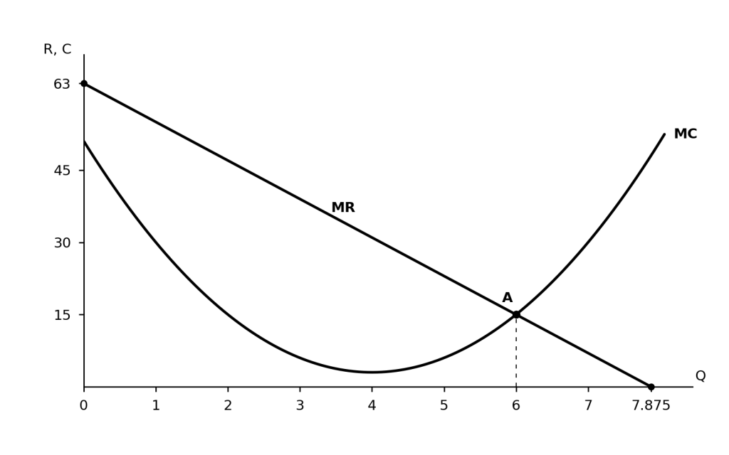
In fact, this depiction of MR and MC more closely resembles the “Nike” curve students are generally familiar with.
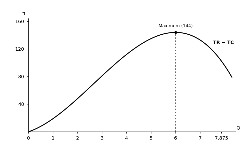
For Q < 6, MR > MC. Therefore, as Q increases, π is continually increasing, reaching its maximum when MR = MC, before falling thereafter since MR < MC. We can see this clearly by plotting profits, π = TR – TC, for this case:
Subnormal profit while profit-maximising.
Students should be aware that achieving profit maximisation does not guarantee that the firm earns supernormal profit, since producing at that quantity may still yield a subnormal profit.
For example, suppose the firm incurs an additional fixed cost of $150. This shifts the TC curve up by 150 and the π curve down by the same amount at every output. MC remains unchanged because fixed cost does not vary with output. It therefore does not affect the cost of producing one more unit.
At the profit-maximising output of Q = 6, economic profit becomes negative, falling from $144 to −$6. The firm’s short-run shutdown decision depends on whether its total revenue covers its total variable costs, as covered in my previous article.
Interestingly, in this case, the firm will continue producing in the short run because average revenue ($39) exceeds average variable cost ($15). It covers its variable costs and puts the remaining revenue towards its fixed costs. By producing, it loses only $6. If it shuts down, it still has to pay its fixed costs of $150.
Conclusion
The lesson for students is to look beyond MC = MR. Check that MC crosses MR from below, so that profit rises before that output and falls after it.
Remember, too, that maximising profit does not necessarily mean earning a positive profit. A firm may be doing the best it can and still make a loss—and whether it continues producing in the short run depends on whether its revenue covers its variable costs.